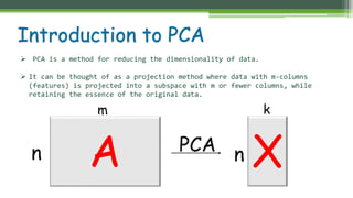
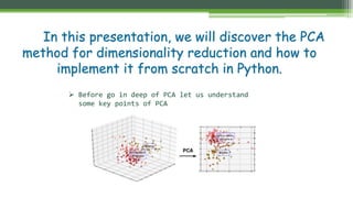
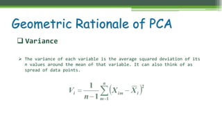
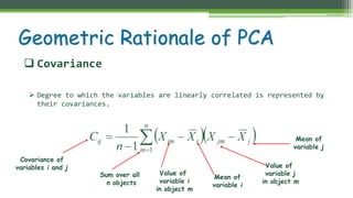
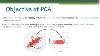
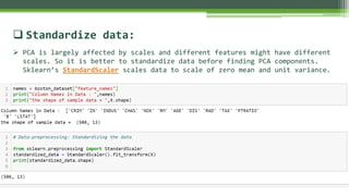
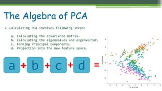
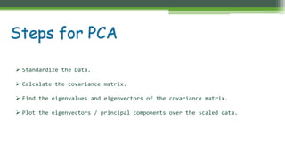
Principal Component Analysis (PCA) and LDA PPT SlidesAbhishekKumar4995
Machine learning (ML) technique use for Dimension reduction, feature extraction and analyzing huge amount of data are Principal Component Analysis (PCA) and Linear Discriminant Analysis (LDA) are easily and interactively explained with scatter plot graph , 2D and 3D projection of Principal components(PCs) for better understanding.
Principal Component Analysis, or PCA, is a factual method that permits you to sum up the data contained in enormous information tables by methods for a littler arrangement of "synopsis files" that can be all the more handily envisioned and broke down.
Naive Bayes is a kind of classifier which uses the Bayes Theorem. It predicts membership probabilities for each class such as the probability that given record or data point belongs to a particular class.
This presentation was prepared as part of the curriculum studies for CSCI-659 Topics in Artificial Intelligence Course - Machine Learning in Computational Linguistics.
It was prepared under guidance of Prof. Sandra Kubler.
In this presentation is given an introduction to Bayesian networks and basic probability theory. Graphical explanation of Bayes' theorem, random variable, conditional and joint probability. Spam classifier, medical diagnosis, fault prediction. The main software for Bayesian Networks are presented.
Lecture 4 Decision Trees (2): Entropy, Information Gain, Gain RatioMarina Santini
attribute selection, constructing decision trees, decision trees, divide and conquer, entropy, gain ratio, information gain, machine leaning, pruning, rules, suprisal
Principal Component Analysis and ClusteringUsha Vijay
Identifying the borrower segments from the give bank data set which has 27000 rows and 77 variable using PROC PRINCOMP. variables, it is important to reduce the data set to a smaller set of variables to derive a feasible
conclusion. With the effect of multicollinearity two or more variables can share the same plane in the in dimensions. Each row of the data can
be envisioned as a 77 dimensional graph and when we project the data as orthonormal, it is expected that the certain characteristics of the
data based on the plots to cluster together as principal components. In order to identify these principal components. PROC PRINCOMP is
executed with all the variables except the constant variables(recoveries and collection fees) and we derive a plot of Eigen values of all the
principal components
Exploratory data analysis in R - Data Science ClubMartin Bago
How to analyse new dataset in R? What libraries to use, and what commands? How to understand your dataset in few minutes? Read my presentation for Data Science Club by Exponea and find out!
Dimensionality Reduction and feature extraction.pptxSivam Chinna
Dimensionality reduction, or dimension reduction, is the transformation of data from a high-dimensional space into a low-dimensional space so that the low-dimensional representation retains some meaningful properties of the original data, ideally close to its intrinsic dimension.
The aim of this report is to use eigenvectors, eigenvalues, and orthogonality to understand the concept of Principal Component Analysis (PCA) and to show why PCA is useful.
Techniques to optimize the pagerank algorithm usually fall in two categories. One is to try reducing the work per iteration, and the other is to try reducing the number of iterations. These goals are often at odds with one another. Skipping computation on vertices which have already converged has the potential to save iteration time. Skipping in-identical vertices, with the same in-links, helps reduce duplicate computations and thus could help reduce iteration time. Road networks often have chains which can be short-circuited before pagerank computation to improve performance. Final ranks of chain nodes can be easily calculated. This could reduce both the iteration time, and the number of iterations. If a graph has no dangling nodes, pagerank of each strongly connected component can be computed in topological order. This could help reduce the iteration time, no. of iterations, and also enable multi-iteration concurrency in pagerank computation. The combination of all of the above methods is the STICD algorithm. [sticd] For dynamic graphs, unchanged components whose ranks are unaffected can be skipped altogether.
Show drafts
volume_up
Empowering the Data Analytics Ecosystem: A Laser Focus on Value
The data analytics ecosystem thrives when every component functions at its peak, unlocking the true potential of data. Here's a laser focus on key areas for an empowered ecosystem:
1. Democratize Access, Not Data:
Granular Access Controls: Provide users with self-service tools tailored to their specific needs, preventing data overload and misuse.
Data Catalogs: Implement robust data catalogs for easy discovery and understanding of available data sources.
2. Foster Collaboration with Clear Roles:
Data Mesh Architecture: Break down data silos by creating a distributed data ownership model with clear ownership and responsibilities.
Collaborative Workspaces: Utilize interactive platforms where data scientists, analysts, and domain experts can work seamlessly together.
3. Leverage Advanced Analytics Strategically:
AI-powered Automation: Automate repetitive tasks like data cleaning and feature engineering, freeing up data talent for higher-level analysis.
Right-Tool Selection: Strategically choose the most effective advanced analytics techniques (e.g., AI, ML) based on specific business problems.
4. Prioritize Data Quality with Automation:
Automated Data Validation: Implement automated data quality checks to identify and rectify errors at the source, minimizing downstream issues.
Data Lineage Tracking: Track the flow of data throughout the ecosystem, ensuring transparency and facilitating root cause analysis for errors.
5. Cultivate a Data-Driven Mindset:
Metrics-Driven Performance Management: Align KPIs and performance metrics with data-driven insights to ensure actionable decision making.
Data Storytelling Workshops: Equip stakeholders with the skills to translate complex data findings into compelling narratives that drive action.
Benefits of a Precise Ecosystem:
Sharpened Focus: Precise access and clear roles ensure everyone works with the most relevant data, maximizing efficiency.
Actionable Insights: Strategic analytics and automated quality checks lead to more reliable and actionable data insights.
Continuous Improvement: Data-driven performance management fosters a culture of learning and continuous improvement.
Sustainable Growth: Empowered by data, organizations can make informed decisions to drive sustainable growth and innovation.
By focusing on these precise actions, organizations can create an empowered data analytics ecosystem that delivers real value by driving data-driven decisions and maximizing the return on their data investment.
Opendatabay - Open Data Marketplace.pptxOpendatabay
Opendatabay.com unlocks the power of data for everyone. Open Data Marketplace fosters a collaborative hub for data enthusiasts to explore, share, and contribute to a vast collection of datasets.
First ever open hub for data enthusiasts to collaborate and innovate. A platform to explore, share, and contribute to a vast collection of datasets. Through robust quality control and innovative technologies like blockchain verification, opendatabay ensures the authenticity and reliability of datasets, empowering users to make data-driven decisions with confidence. Leverage cutting-edge AI technologies to enhance the data exploration, analysis, and discovery experience.
From intelligent search and recommendations to automated data productisation and quotation, Opendatabay AI-driven features streamline the data workflow. Finding the data you need shouldn't be a complex. Opendatabay simplifies the data acquisition process with an intuitive interface and robust search tools. Effortlessly explore, discover, and access the data you need, allowing you to focus on extracting valuable insights. Opendatabay breaks new ground with a dedicated, AI-generated, synthetic datasets.
Leverage these privacy-preserving datasets for training and testing AI models without compromising sensitive information. Opendatabay prioritizes transparency by providing detailed metadata, provenance information, and usage guidelines for each dataset, ensuring users have a comprehensive understanding of the data they're working with. By leveraging a powerful combination of distributed ledger technology and rigorous third-party audits Opendatabay ensures the authenticity and reliability of every dataset. Security is at the core of Opendatabay. Marketplace implements stringent security measures, including encryption, access controls, and regular vulnerability assessments, to safeguard your data and protect your privacy.
Adjusting primitives for graph : SHORT REPORT / NOTESSubhajit Sahu
Graph algorithms, like PageRank Compressed Sparse Row (CSR) is an adjacency-list based graph representation that is
Multiply with different modes (map)
1. Performance of sequential execution based vs OpenMP based vector multiply.
2. Comparing various launch configs for CUDA based vector multiply.
Sum with different storage types (reduce)
1. Performance of vector element sum using float vs bfloat16 as the storage type.
Sum with different modes (reduce)
1. Performance of sequential execution based vs OpenMP based vector element sum.
2. Performance of memcpy vs in-place based CUDA based vector element sum.
3. Comparing various launch configs for CUDA based vector element sum (memcpy).
4. Comparing various launch configs for CUDA based vector element sum (in-place).
Sum with in-place strategies of CUDA mode (reduce)
1. Comparing various launch configs for CUDA based vector element sum (in-place).
Chatty Kathy - UNC Bootcamp Final Project Presentation - Final Version - 5.23...John Andrews
SlideShare Description for "Chatty Kathy - UNC Bootcamp Final Project Presentation"
Title: Chatty Kathy: Enhancing Physical Activity Among Older Adults
Description:
Discover how Chatty Kathy, an innovative project developed at the UNC Bootcamp, aims to tackle the challenge of low physical activity among older adults. Our AI-driven solution uses peer interaction to boost and sustain exercise levels, significantly improving health outcomes. This presentation covers our problem statement, the rationale behind Chatty Kathy, synthetic data and persona creation, model performance metrics, a visual demonstration of the project, and potential future developments. Join us for an insightful Q&A session to explore the potential of this groundbreaking project.
Project Team: Jay Requarth, Jana Avery, John Andrews, Dr. Dick Davis II, Nee Buntoum, Nam Yeongjin & Mat Nicholas
2. How do we choose the
right features ?
Given a
classification
problem ….
3. PCA is a method for reducing the dimensionality of data.
It can be thought of as a projection method where data with m-columns
(features) is projected into a subspace with m or fewer columns, while
retaining the essence of the original data.
An PCA
Xn
km
Introduction to PCA
4. In this presentation, we will discover the PCA
method for dimensionality reduction and how to
implement it from scratch in Python.
Before go in deep of PCA let us understand
some key points of PCA
5. Variance
The variance of each variable is the average squared deviation of its
n values around the mean of that variable. It can also think of as
spread of data points.
Geometric Rationale of PCA
6. Covariance
Covariance of
variables i and j
Sum over all
n objects
Value of
variable i
in object m
Mean of
variable i
Value of
variable j
in object m
Mean of
variable j
Degree to which the variables are linearly correlated is represented by
their covariances.
Geometric Rationale of PCA
7. Objective of PCA
Objective of PCA is to rigidly rotate the axes of this m-dimensional space to new positions
(principal axes)
PCA is ordered such that principal axis 1 has the highest variance, axis 2 has the next
highest variance .... , and axis p has the lowest variance
8. Implement PCA in Python (Scratch)
Load the Data-Set :
We can use Boston Housing dataset for PCA. Boston dataset has 13
features. So question here is how to visualize the data ?. We can
reduce the dimensions of data by using PCA and then visualize.
9. Standardize data:
PCA is largely affected by scales and different features might have different
scales. So it is better to standardize data before finding PCA components.
Sklearn’s StandardScaler scales data to scale of zero mean and unit variance.
10. The Algebra of PCA
Calculating PCA involves following steps:
a. Calculating the covariance matrix.
b. Calculating the eigenvalues and eigenvector.
c. Forming Principal Components.
d. Projection into the new feature space.
a b dc+ + ++ =
11. Calculating the covariance matrix (S) :
Covariance matrix is a matrix of variances and covariances (or correlations) among
every pair of the m variables .
It is square, symmetric matrix.
Covariance matrix (S) = X.T * X, we can find it by using numpy matmul() function
in python.
12. Calculating the eigenvalues and eigenvector :
ƛ is an eigenvalue for a matrix X if it is a solution of the characteristic
equation:
det( ƛ*I - A ) = 0
Where, I is the identity matrix of the same dimension as X.
The sum of all m eigenvalues equals the trace of S (the sum of the variances of
the original variables).
13. For each eigenvalue ƛ, a corresponding eigen-vector v, can be found by
solving :
( ƛ*I - A )v = 0
The eigenvalues, 1, 2, ... m are the variances of the coordinates
on each principal component axis.
Calculating the eigenvalues and eigenvector :
14. We are using scipy.linalg, which have eigh function for finding the top eigen-
values & eigen-vector, we are finding top 2 eigenvalues and eigenvectors as follow.
Code for finding eigenvalues and eigenvector :
15. Forming Principal Components :
Below is code for forming principal components, formed by two principal eigen
vectors by vector-vector multiplication
16. Projection into the new feature space :
Creating a Data Frame having 1st principal & 2nd Principal components.
18. Steps for PCA
Standardize the Data.
Calculate the covariance matrix.
Find the eigenvalues and eigenvectors of the covariance matrix.
Plot the eigenvectors / principal components over the scaled data.
19. 1) [ True or False ] PCA can be used for projecting and visualizing data in lower
dimensions.
A. TRUE
B. FALSE
2) We apply PCA on image dataset.
A. TRUE
B. FALSE
3) PCA is based on variance maximization and distance minimization.
A. TRUE
B. FALSE
Implement PCA for number of components = 3 and then visualize data, also load
iris dataset and perform same task
Assessment and Evaluation
Ans:1-A,2-A,3-A
20. For full code : https://github.com/Eshan2203/PCA-on-Boston-House-price-Data-
Set/blob/master/PCA_BOston.ipynb
Editor's Notes
How presentation will benefit audience: Adult learners are more interested in a subject if they know how or why it is important to them.
Presenter’s level of expertise in the subject: Briefly state your credentials in this area, or explain why participants should listen to you.
Lesson descriptions should be brief.
Example objectives
At the end of this lesson, you will be able to:
Save files to the team Web server.
Move files to different locations on the team Web server.
Share files on the team Web server.