Sorting and Searching Techniques

For More Visit: Https://www.ThesisScientist.com
Unit 10
Sorting and Searching Techniques
Searching
Information retrieval in the required format is the common activity in all computer applications. This
involves searching, sorting and merging. Searching methods are designed to take advantage of the file
organization and optimize the search for a particular record or establish its absence.
Sequential Search
The simplest technique for searching an unordered table for a particular record is to scan each entry in the
table in a sequential manner until the desired record is found. This is the most natural way of searching. In
this method we simply go through a list or a file till the required record is found or end of list or file is
encountered. Ordering of list is not important.
Efficiency of Sequential Search
Let us assume that there no insertion and deletion are made i.e. we are searching through a table of constant
size n. If the record we are searching is the first one in the table, only one comparison is performed. If the
record is the last one in the table, n comparisons are necessary. Hence, the average number of comparisons
done by sequential search are:
1+2+3 .. + I + .. +N
N
N (N+1)
2 * N
N+1
2
Sequential search is easy to write and efficient for short list. It does not require sorted data. It is disastrous
for long lists.
Binary Search
Another relatively simple method of accessing a table is the binary search method. The entries in the table
are stored in alphabetically or numerically increasing order.
The drawback of sequential search can be eliminated if it becomes possible to eliminate large portions of
the list from consideration in subsequent iterations. Binary search requires sorted data to operate on. In this
method, search begins by examining the records in the middle of file rather than the one at one of the ends
as in sequential search.

Let us assume that file being searched is sorted on increasing value of key. Based on the result of the
comparison with the middle key, Km, following conclusion can be drawn.
 If K < Km then if the record being searched for is in the file, it must be in the lower numbered half
of the file.
 If K = Km then the middle record is the one being searched for.
 If K > Km then if the record being searched for is in the file it must be in the higher numbered half
of the file.
Efficiency of Binary Search
Each comparison in the binary search reduces the number of possible candidates by a factor of 2. Thus, the
maximum number of key comparisons is approximately log2n. Therefore, the binary search algorithm is
O(log n).
Indexed Sequential Search
This method increases the amount of space required for searching. In this method an auxiliary table, called
an index is created in addition to the stored file itself. Each element in the index consists of a key KINDEX
and a pointer to the record in the file that corresponds to KINDEX.
The elements in the index, as well as the elements in the file, must be sorted on the key. If the index is one-
third the size of the file, every third record of the file is represented in the index.

115
530
561
8
14
20
38
72
115
421
436
530
532
549
561
563
650
Index Kind
P index
k
(Index)
r
(Record)
115
530
561
8
14
20
38
72
115
421
436
530
532
549
561
563
650
Index Kind
P index
k
(Index)
r
(Record)
Figure 10.1: Indexed Sequential File
Assume that k is the key field and key is the value being searched (figure 10.1). Also, let kindex be an array
of the keys in the index of the record-file and pindex be the array of pointers within the index to the actual
records in the file. Also assume that the file is sorted as an array, that n is the file size and that indxsze is the
size of the index.
Sorting
Sorting refers to the operation of arranging data in some given order, such as increasing or decreasing, with
numerical data or alphabetically, with character data.
Let P be a list of n elements P1, P2, P3...Pn in memory. Sorting P refers to the operation of rearranging the
contents of P so that they are increasing in order (numerically or lexicographically), that is,
P1 < P2 < P3...< Pn
Since P has n elements, there are n! ways that the contents can appear in P. These ways correspond
precisely to the n! permutations of 1, 2, ...n. Accordingly, each sorting algorithm must take care of these n!
possibilities.

'O' Notation
Given two functions f(n) and g(n), we say that f(n) is of the order of g(n) or that f(n) is O(g(n)) if there
exists positive integers a and b such that
f(n)  a * g (n) for n  b.
For example, if f(n) = n2
+ 100n and g (n) = n2
f(n) is O(g(n)), since n2
+ 100n
is less than or equal to 2n2
for all n greater than or equal to 100. In this case a = 2 and b = 100.
Bubble Sort
Another well known sorting method is the Bubble Sort. In this approach, there are at most n-1 passes
required.
In bubble sort, the file is passed through sequentially several times. In each pass each element is compared
with its successor. i.e (x[i] with x [i+1] and interchanged if they are not in the proper order.
Example
The following comparisons are made on the first pass :
x[0] with x[1] (25 with 57) No interchange
x[1] with x[2] (57 with 48) Interchange
x[4] with x[5] (57 with 92) No Interchange
Thus after the first pass, the file is in the order
25, 48, 37, 12, 57, 86, 33, 92
After first pass, the largest element (92) is in its proper position within the array. In general, x[n-i] will be
in its proper position after insertion i. The complete set of iterations are as follows :
iteration 0 (original file) 25 57 48 37 12 92 86 33
Iteration 1 25 48 37 12 57 86 33 92
Iteration 2 25 37 12 48 57 33 86 92
Iteration 3 25 12 37 48 33 57 86 92
Iteration 4 12 25 37 33 48 57 86 92
Iteration 5 12 25 33 37 48 57 86 92
Iteration 6 12 25 33 37 48 57 86 92
Iteration 7 12 25 33 37 48 57 86 92

Since all the elements in position greater than or equal to n-i are already in proper position after iteration i,
they need not be considered in succeeding iterations. Thus, on the first pass n-1 comparisons are made, on
the second pass n-2 comparisons are made, and on the (n-1)th
pass only one comparison is made (between
x[0] and x[1]. This enhancement speeds up the process.
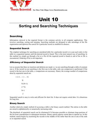
Although n-1 passes are required to sort a file, however, in the preceding example the file was sorted after
five iterations making the last two iterations unnecessary. To eliminate the unnecessary passes we keep a
record of whether or not any interchange is made in a given pass, so that further passes can be eliminated.
Unsorted Pass Number (i) Sorted
j Kj 1 2 3 4 5 6
1 42 23 23 11 11 11 11
2 23 42 11 23 23 23 23
3 74 11 42 42 42 36 36
4 11 65 58 58 36 42 42
5 65 58 65 36 58 58 58
6 58 74 36 65 65 65 65
7 94 36 74 74 74 74 74
8 36 94 87 87 87 87 87
9 99 87 94 94 94 94 94
10 87 99 99 99 99 99 99
Unsorted Pass Number (i) Sorted
j Kj 1 2 3 4 5 6
1 42 23 23 11 11 11 11
2 23 42 11 23 23 23 23
3 74 11 42 42 42 36 36
4 11 65 58 58 36 42 42
5 65 58 65 36 58 58 58
6 58 74 36 65 65 65 65
7 94 36 74 74 74 74 74
8 36 94 87 87 87 87 87
9 99 87 94 94 94 94 94
10 87 99 99 99 99 99 99
Figure 10.2: Trace of a bubble sort
Efficiency of Bubble Sort
Considering no improvements are made:
 There are n-1 passes and n-1 comparisons on each pass.
 Thus the total number of comparisons are (n-1) (n-1) = n2
-2n+1 which is O(n2
).
 Considering the improvements

 If there are k iterations the total number of comparisons are (n-1) + (n-2) + (n-3) + .. + (n-k), which
equals (2nk – k2
- k) /2.
Quick Sort
Quick sort is also known as partition exchange sort. An element (a) is chosen from a specific position
within the array such that x is partitioned and a is placed at position j and the following conditions hold:
1. Each of the elements in position 0 through j-1 is less than or equal to a.
2. Each of the elements in position j+1 through n-1 is greater than or equal to a.
The purpose of the Quick Sort is to move a data item in the correct direction just enough for it to reach its
final place in the array. The method, therefore reduces unnecessary swaps, and moves an item a great
distance in one move. A pivotal item near the middle of the array is chosen, and then items on either side
are moved so that the data items on one side of the pivot are smaller than the pivot, whereas those on the
other side are larger. The middle (pivot) item is in its correct position. The procedure is then applied
recursively to the parts of the array, on either side of the pivot, until the whole array is sorted.
Example
If an initial array is given as:
25 57 48 37 12 92 86 33
and the first element (25) is placed in its proper position, the resulting array is :
12 25 57 48 37 92 86 33
At this point, 25 is in its proper position in the array (x[1]), each element below that position (12) is less
than or equal to 25, and each element above that position (57, 40, 37, 92 86 and 33) is greater than or equal
to 25.
Since 25 is in its final position the original problem has been decomposed into the problem of sorting the
two sub-arrays.
(12) and (57 48 37 92 86 33)
First of these sub-arrays has one element so there is no need to sort it. Repeating the process on the sub-
array x[2] through x[7] yields :
12 25 (48 37 33) 57 (92 86)
and further repetitions yield
12 25 (37 33) 48 57 (92 86)
12 25 (33) 37 48 57 (92 86)
12 25 33 37 48 57 (92 86)
12 25 33 37 48 57 (86) 92
12 25 33 37 48 57 86 92

We shall illustrate the mechanics of this method by applying it to an array of numbers. Suppose the array A
initially appears as :
(15, 20, 5, 8, 95, 12, 80, 17, 9, 55)
Figure 10.3 shows a quick sort applied to this array.
A(1) A(2) A(3) A(4) A(5) A(6) A(7) A(8) A(9) A(10)
15 20 5 8 95 12 80 17 9 55
9 20 5 8 95 12 80 17 ( ) 55
9 ( ) 5 8 95 12 80 17 20 55
9 12 5 8 95 ( ) 80 17 20 55
9 12 5 8 ( ) 95 80 17 20 55
9 12 5 8 15 95 80 17 20 55
Figure 10.3 : Quick Sort of an Array
Analysis of Quick Sort
Assumption : i) File is of size n where n is a power of 2.
Say n = 2m
, so that m = log2n.
Selection Sort
One of the easiest ways to sort a table is by selection. Beginning with the first record in the table, a search is
performed to locate the element, if found it is placed as the first record in the table, rest of the records are
shifted by one place. A search for the second smallest key is then carried out. This is accomplished by
examining the keys of the records from the second element onwards. The element, which has the second
smallest key is placed as the second element of the table, rest of the records are shifted by one place. The
process of searching for the record with the next smallest key and placing it in its proper position continues
until all the records have been sorted in ascending order.
A selection sort is one in which successive elements are selected in order and placed into their proper sorted
positions. The elements of the input may have to be preprocessed to make the ordered selection possible.
The basic idea of the selection sort is to repeatedly select the smallest key in the remaining unsorted array.
A general algorithm for the selection sort:
1. Repeat through step 5 a total of n-1 times, n being number of elements to be sorted.
2. Record the position of the table already sorted.
3. Repeat step 4 for the elements in the unsorted position of the table.
4. Record location of smallest element in unsorted table.

5. Place smallest element in the first place of table and shift the array by one place.
Example
Consider the following unsorted array to be sorted using selection sort.
Step 1 : 2 is chosen as it is the smallest element and is put in sorted part at 1st position. Now the array
becomes as:
Step 2 : The second pass identifier 3 is the smallest element in remaining unsorted array. Adding 3 also in
the sorted part at 2nd position we have the following array:
Step 3 : In third pass 6 is chosen as smallest and put at position 3 and the array becomes:
Step 4 :
Step 5 :
Step 6 :
Step 7 :
Therefore, after seventh pass the array is sorted. The above-mentioned technique uses a separate area to
store sorted part; therefore, more space is required to work on it.

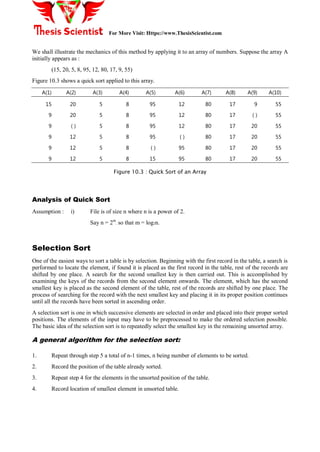
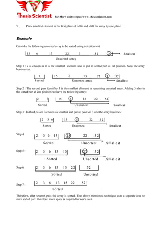
(Exchange) Selection sort
A modification to straight selection sort is the Exchange Selection Sort, where the smallest key is moved
into its final position by being exchanged with the key initially occupying that position.
Figure 22.1: Exchange Selection Sort
Analysis of Selection Sort
The ordering in a selection sort is not important. If an entry is in its correct final position, then it will never
be moved. Every time any pair of entries is swapped, then at least one of them moves into its final position,
and therefore at most n-1 swaps are done altogether in sorting a list of n entries.
The comparison is done for minimum value, with the length of sub list ranging from n down to 2. Thus,
altogether there are:
(n - 1) + (n - 2) + .. + 1 = ½ * n ( n - 1)
comparisons of keys which approximates to
n2
/2 + O (n)
The order of selection sort comes out to be of O(n2
).
Insertion Sort
An insertion sort is one that sorts a set of records by inserting records into an existing sorted file. Suppose
an array A with n elements A[1], A[2],.......A[N] is in memory. The insertion sort algorithm scans A from

A[1] to A[N], inserting each element A[K] into its proper position in the previously sorted sub array A[1],
A[2],... A[K-1].
Example
Sort the following list using the insertion sort method : 4, 1, 3, 2, 5
i) 4 Place 4 in 1st
position
ii) 1 4 1 < 4, therefore insert prior to 4
iii) 1 3 4 3 > 1, insert between 1 & 4
iv) 1 2 3 4 2 > 1, insert between 1 & 3
v) 1 2 3 4 5 5>4, insert after 4
Thus, to find the correct position, search the list till an item just greater than the target is found; shift all the
items from this point one down the list, insert the target in the vacated slot.
Analysis of Insertion Sort
If the initial file is sorted, only one comparison is made on each pass, so that sort is O(n). If the file is
initially sorted in reverse order, the sort is O(n2
), since the total number of comparisons are:
(n-1) + (n-2) + ... + 3 + 2 + 1 = (n-1) * n/2
which is O(n2
).
The closer the file is to sorted order, the more efficient the simple insertion sort becomes. The space
requirements for the sort consists of only one temporary variable, Y. The speed of the sort can be improved
somewhat by using a binary search to find the proper position for x[k] in the sorted file.
x[0], x[1] ... x[k-1]
This reduces the total number of comparisons from O(n2
) to O(n log2 (n
Shell Sort
More significant improvement on simple insertion sort than binary or list insertion can be achieved using
the Shell Sort (Diminishing Increment Sort). This method sorts separate sub-files of the original file.
These sub-files contain every kth
element of the original file. The value of k is called an increment. For
example, if k is 5, the sub-file consisting of x[0], x[5], x[10],... is first sorted. Five sub-files, each
containing the one fifth of the element of the original file are sorted in this manner. These are :
Sub-file 1 : x[0] x[5] x[10] ....
Sub-file 2 : x[1] x[6] x[11] ....
Sub-file 3 : x[2] x[7] x[12] ....
Sub-file 4 : x[3] x[8] x[13] ...
Sub-file 5 : x[4] x[9] x[14] ...
The ith
element of the jth
sub-file is x[(i-1)* 5+j-1]. If a different increment is chosen, the k sub-files are
divided so that the ith
element of the jth
sub-file is x[(i-1) * k+j-1].

A decreasing sequence of increments is fixed at the start of the entire process. The last value in this
sequence must be 1.
Example
The following figure illustrates the shell sort on this sample file:
Original file: [25 57 48 37 12 92 86 33]
Pass 1 25 57 48 37 12 92 86 33
Span = 5
Pass 2 25 57 33 37 12 92 86 48
Span 3
Pass 3 25 12 33 37 48 92 86 57
Span = 1
Sorted file 12 25 33 37 48 57 86 92
Analysis of Shell Sort
Since the first increment used by the shell sort is large, the individual sub-files are quite small, so that the
simple insertion sort on those sub-files are fairly fast. Each sort of a sub-file causes the entire file to be
more nearly sorted. Thus although successive passes of the shell sort use smaller increments and therefore
deal with larger sub-files. Those sub-files are almost sorted due to the actions of previous passes.
Thus the insertion sort on these sub-files are also quite efficient. The actual time requirement for a specific
sort depends on the number of elements in the array increments and on their actual values.
It has been shown that order of the shell sort can be approximated by O(n * (log (n2
))
Merge sort
The operation of sorting is closely related to the process of merging. This sorting method uses merging of
two ordered arrays, which can be combined to produce a single sorted array. This process can be
accomplished easily by successively selecting the record with the smallest key occurring in either of the
arrays and placing this record in a new table, thereby creating an ordered array.
Merge sort is one of the divide and conquer class of algorithm. The basic idea is:
 Divide the array to a number of sub-arrays.
 Sort each of these sub-arrays.
 Merge them to get a single sorted array.
2-way merge sort divides the list into two sorted sub-arrays and then merges them to get the sorted array,
also called concatenate sort.
Multiple merging can also be accomplished by performing a simple merge repeatedly. For example if we
have 16 arrays to merge, we can first merge them in pairs. The result of this first step yields eight tables,
which are again merged in pairs to give four tables. This process is repeated until a single table is obtained.

In this example four separate passes are required to yield a single list. In general, k separate passes are
required to merge 2k separate lists into a single list.
Example
i [7] [4] [1] [3] [0] [2] [6] [5]
ii [4 7] [1 3] [0 2] [5 6]
iii [1 3 4 7] [0 2 5 6]
iv [0 1 2 3 4 5 6 7]
The format statement of above method is as follows:
Analysis of Merge Sort
Analysis of procedure merge
Analysis of routine that uses procedure merge
For an array of size N, on the ith
pass the files being merged are of size 2i-1
. Consequently, a total of log2(N)
passes are made over the data. Since two files can be merged in linear time (algorithm merge), each pass of
merge sort takes O(N) time. As there are [log2 (N)] passes, the total computing time is O(N * log2 N).

Sorting and Searching Techniques

Recommended

Recommended

More Related Content

What's hot

What's hot (20)

Similar to Sorting and Searching Techniques

Similar to Sorting and Searching Techniques (20)

More from Prof Ansari

More from Prof Ansari (20)

Recently uploaded

Recently uploaded (20)

Sorting and Searching Techniques