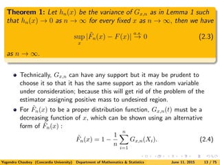
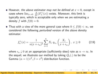
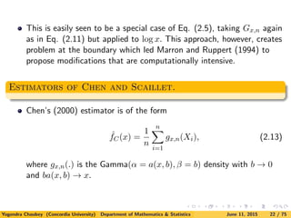
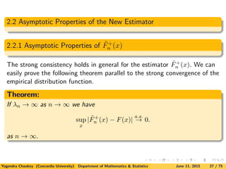
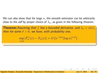
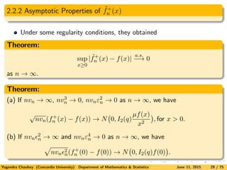
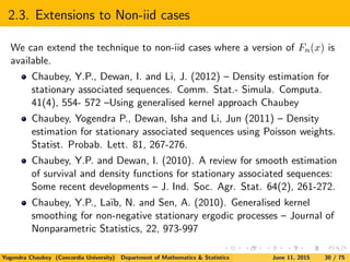
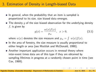
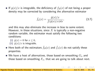
- The document discusses nonparametric density estimation for data with non-negative support, such as data from reliability testing.
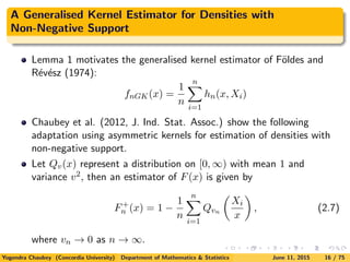
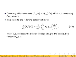
- It proposes several density estimators based on an approximation lemma, including using asymmetric kernels and distributions placed on lattice points.
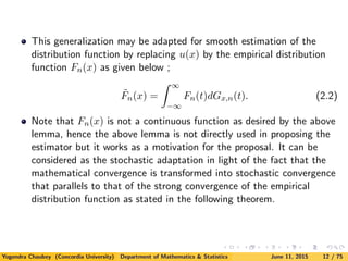
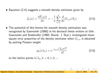
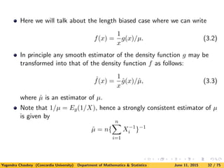
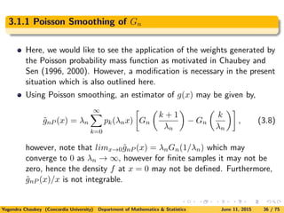
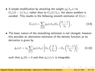
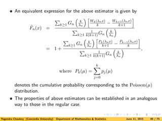
- The estimators are motivated by replacing the empirical distribution function in the lemma with a smoothed version, yielding a smoothed density estimator.
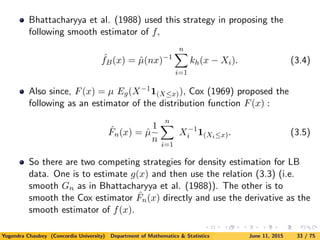
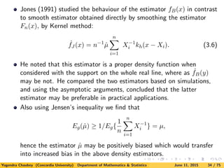
- Asymptotic properties of the estimators are established, and simulations compare their performance.

![Abstract
This talk will highlight some recent developments in the area of
nonparametric functional estimation with emphasis on nonparametric
density estimation for size biased data. Such data entail constraints that
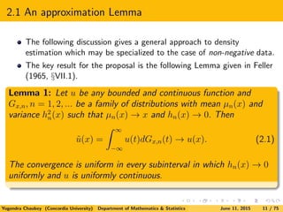
many traditional nonparametric density estimators may not satisfy. A
lemma attributed to Hille, and its generalization [see Lemma 1, Feller
(1965) An Introduction to Probability Theory and Applications, §VII.1)] is
used to propose estimators in this context from two different perspectives.
After describing the asymptotic properties of the estimators, we present
the results of a simulation study to compare various nonparametric density
estimators. The optimal data driven approach of selecting the smoothing
parameter is also outlined.
Yogendra Chaubey (Concordia University) Department of Mathematics & Statistics June 11, 2015 2 / 75](https://image.slidesharecdn.com/slides-csm-150611013053-lva1-app6892/85/Slides-csm-2-320.jpg)
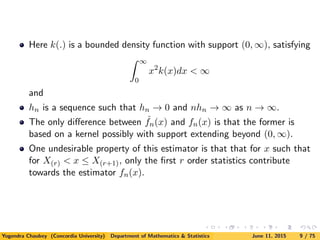
![Based on a random sample (X1, X2, ..., Xn), from a univariate
density f(.), the empirical distribution function (edf) is defined as
Fn(x) =
1
n
n
i=1
I(Xi ≤ x). (1.2)
edf is not smooth enough to provide an estimator of f(x).
Various methods (viz., kernel smoothing, histogram methods, spline,
orthogonal functionals)
The most popular is the Kernel method (Rosenblatt, 1956).
[See the text Nonparametric Functional Estimation by Prakasa Rao
(1983) for a theoretical treatment of the subject or Silverman (1986)].
Yogendra Chaubey (Concordia University) Department of Mathematics & Statistics June 11, 2015 5 / 75](https://image.slidesharecdn.com/slides-csm-150611013053-lva1-app6892/85/Slides-csm-5-320.jpg)
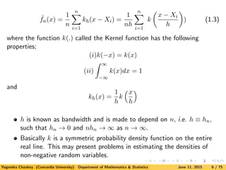
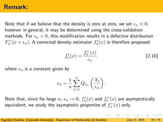
![1.2. Smooth Estimation of densities on R+
ˆfn(x) might take positive values even for x ∈ (−∞, 0], which is not
desirable if the random variable X is positive. Silverman (1986)
mentions some adaptations of the existing methods when the support
of the density to be estimated is not the whole real line, through
transformation and other methods.
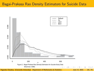
1.2.1 Bagai-Prakasa Rao Estimator
Bagai and Prakasa Rao (1996) proposed the following adaptation of
the Kernel Density estimator for non-negative support [which does
not require any transformation or corrective strategy].
fn(x) =
1
nhn
n
i=1
k
x − Xi
hn
, x ≥ 0. (1.4)
Yogendra Chaubey (Concordia University) Department of Mathematics & Statistics June 11, 2015 8 / 75](https://image.slidesharecdn.com/slides-csm-150611013053-lva1-app6892/85/Slides-csm-8-320.jpg)
![Other developments:
This lemma has been further used to motivate the Bernstein
Polynomial estimator (Vitale, 1975) for densities on [0, 1] by Babu,
Canty and Chaubey (1999). Gawronski (1985, Period. Hung.)
investigates other lattice distributions such as negative binomial
distribution.
Some other developments:
Chaubey and Sen (1996, Statist. Dec.): survival functions, though in a
truncated form.
Chaubey and Sen (1999, JSPI): Mean Residual Life; Chaubey and Sen
(1998a, Persp. Stat., Narosa Pub.): Hazard and Cumulative Hazard
Functions; Chaubey and Sen (1998b): Censored Data;
(Chaubey and Sen, 2002a, 2002b): Multivariate density estimation
Smooth density estimation under some constraints: Chaubey and
Kochar (2000, 2006); Chaubey and Xu (2007, JSPI).
Babu and Chaubey (2006): Density estimation on hypercubes. [see
also Prakasa Rao(2005)and Kakizawa (2011), Bouezmarni et al. (2010,
JMVA) for Generalised Bernstein Polynomials and Bernstein copulas]
Yogendra Chaubey (Concordia University) Department of Mathematics & Statistics June 11, 2015 15 / 75](https://image.slidesharecdn.com/slides-csm-150611013053-lva1-app6892/85/Slides-csm-15-320.jpg)
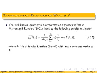
![It may also be remarked that the idea used here may be extended to
the case of densities supported on an arbitrary interval
[a, b], − ∞ < a < b < ∞, by choosing for instance a Beta kernel
(extended to the interval [a, b]) as in Chen (1999). Without loss of
generality, suppose a = 0 and b = 1. Then we can choose, for
instance, qv(.) as the density of Y/µ, where
Y ∼ Beta(α, β), µ = α/(α + β), such that α → ∞ and β/α → 0, so
that Var(Y/µ) → 0.
Yogendra Chaubey (Concordia University) Department of Mathematics & Statistics June 11, 2015 26 / 75](https://image.slidesharecdn.com/slides-csm-150611013053-lva1-app6892/85/Slides-csm-26-320.jpg)
![Since,
∞
0
˜gn(x)
x
dx = λn
k≥1
[Gn
k
λn
− Gn
k − 1
λn
]
∞
0
pk(xλn)
x
dx
= λn
k≥1
[Gn
k
λn
− Gn
k − 1
λn
]
1
k
= λn
k≥1
1
k(k + 1)
Gn
k
λn
,
The new smooth estimator of the length biased density f(x) is given
by
˜fn(x) =
k≥1
pk−1(xλn)
k Gn
k
λn
− Gn
k−1
λn
k≥1
1
k(k+1) Gn
k
λn
. (3.11)
Yogendra Chaubey (Concordia University) Department of Mathematics & Statistics June 11, 2015 38 / 75](https://image.slidesharecdn.com/slides-csm-150611013053-lva1-app6892/85/Slides-csm-38-320.jpg)
![The corresponding smooth estimator of the distribution function
F(x) is given by
˜Fn(x) =
k≥1(1/k)Wk(xλn)[Gn
k
λn
− Gn
k−1
λn
]
k≥1
1
k(k+1)Gn
k
λn
(3.12)
where
Wk(λnx) =
1
Γ(k)
λnx
0
e−y
yk−1
dy =
j≥k
pj(λnx).
Yogendra Chaubey (Concordia University) Department of Mathematics & Statistics June 11, 2015 39 / 75](https://image.slidesharecdn.com/slides-csm-150611013053-lva1-app6892/85/Slides-csm-39-320.jpg)

![4. Choice of Smoothing Parameters
4.2 Biased Cross Validation
This criterion involves minimization of an estimate of the asymptotic
mean integrated squared error (AMISE).
For AMISE( ˆfn), we use the formula as obtained in Chaubey et al.
(2012), that is given by
AMISE[ ˆf+
n (x)] =
I2(q)µ
nvn
∞
0
f(x)
(x + εn)2
dx
+
∞
0
[v2
nf(x) + (2v2
nx + εn)f (x) + v2
n
x2
2
f (x)]2
dx
(4.1)
where I2(q) lim
v→0
v
∞
0 (qvn (t))2dt.
Yogendra Chaubey (Concordia University) Department of Mathematics & Statistics June 11, 2015 46 / 75](https://image.slidesharecdn.com/slides-csm-150611013053-lva1-app6892/85/Slides-csm-46-320.jpg)
![4. Choice of Smoothing Parameters
4.2 Biased Cross Validation
The AMISE( ˜fn), is given by in Chaubey et al. (2012), that is given
by
AMISE[ ˜f+
n ] =
∞
0
[(xv2
n + εn)f (x) +
x2
2
f (x)v2
n]2
dx
+
I2(q)µ
nvn
∞
0
f(x)
(x + εn)2
dx.
(4.2)
The Biased Cross Validation (BCV) criterion is defined as
BCV (vn, εn) = AMISE(fn). (4.3)
Yogendra Chaubey (Concordia University) Department of Mathematics & Statistics June 11, 2015 47 / 75](https://image.slidesharecdn.com/slides-csm-150611013053-lva1-app6892/85/Slides-csm-47-320.jpg)
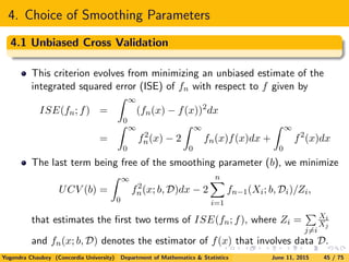
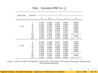
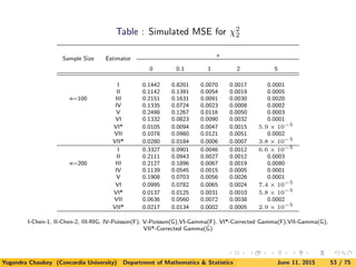
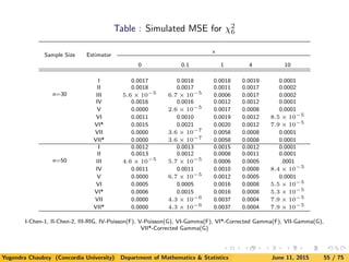
![5. A Simulation Study
Here we consider parent distributions to estimate as exponential (χ2
2),
χ2
6, lognormal, Weibull and mixture of exponential densities.
Since the computation is very extensive for obtaining the smoothing
parameters, we compute approximations to MISE and MSE by
computing
ISE(fn, f) =
∞
0
[fn(x) − f(x)]2
dx
and
SE (fn(x), f(x)) = [fn(x) − f(x)]2
for 1000 samples.
Yogendra Chaubey (Concordia University) Department of Mathematics & Statistics June 11, 2015 48 / 75](https://image.slidesharecdn.com/slides-csm-150611013053-lva1-app6892/85/Slides-csm-48-320.jpg)
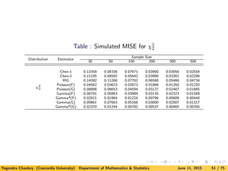
![Next table gives the values of MISE for exponential density using new
estimators as compared with Chen’s and Scaillet estimators. Note
that we include the simulation results for Scaillet’s estimator using
RIG kernel only.
Inverse Gaussian kernel is known not to perform well for direct data
[see Kulasekera and Padgett (2006)]. Similar observations were noted
for LB data.
Yogendra Chaubey (Concordia University) Department of Mathematics & Statistics June 11, 2015 50 / 75](https://image.slidesharecdn.com/slides-csm-150611013053-lva1-app6892/85/Slides-csm-50-320.jpg)

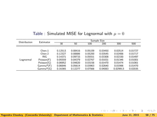
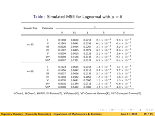
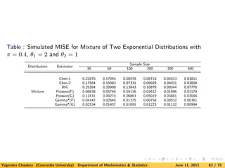
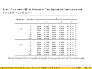
![We have considered following additional distributions for simulation as well:
(i). Lognormal Distribution
f(x) =
1
√
2πx
exp{−(log x − µ)2
/2}I{x > 0};
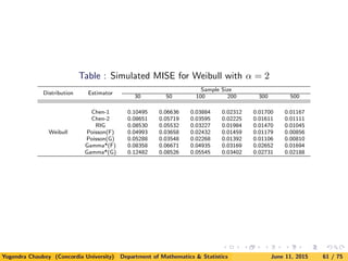
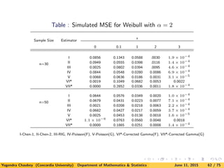
(ii). Weibull Distribution
f(x) = αxα−1
exp(−xα
)I{x > 0};
(iii). Mixtures of Two Exponential Distribution
f(x) = [π
1
θ1
exp(−x/θ1) + (1 − π)
1
θ2
exp(−x/θ2]I{x > 0}.
Yogendra Chaubey (Concordia University) Department of Mathematics & Statistics June 11, 2015 57 / 75](https://image.slidesharecdn.com/slides-csm-150611013053-lva1-app6892/85/Slides-csm-57-320.jpg)