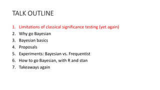
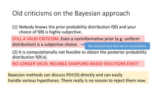
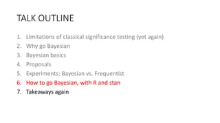
Download as PDF, PPTX

![1. P-values can indicate how incompatible the data are with a
specified statistical model.
2. P-values do not measure the probability that the studied
hypothesis is true, or the probability that the data were
produced by random chance alone.
3. Scientific conclusions and business or policy decisions
should not be based only on whether a p-value passes a
specific threshold.
[Wasserstein+16]](https://image.slidesharecdn.com/sigir2017bayesian-170808065151/85/sigir2017bayesian-4-320.jpg)
![4. Proper inference requires full reporting and transparency.
5. A p-value, or statistical significance, does not measure the
size of an effect or the importance of a result.
6. By itself, a p-value does not provide a good measure of
evidence regarding a model or hypothesis.
P-value = P(D+|H)
Probability of observing the observed data D or
something more extreme UNDER Hypothesis H.
[Wasserstein+16]](https://image.slidesharecdn.com/sigir2017bayesian-170808065151/85/sigir2017bayesian-5-320.jpg)
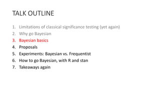
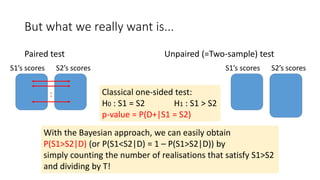
![Problems with classical significance testing
• Statistical significance ≠ practical significance
• Dichotomous thinking: statistically significant (p<0.05) or not
• P-values and CIs are often misunderstood (see the ASA statements)
• Even if the p-value is reported, p-value = f(effect_size, sample_size)
large effect_size (magnitude of difference) ⇒ small p-value
large sample_size (e.g. #topics) ⇒ small p-value.
So effect sizes should be reported [Sakai14SIGIRforum].
“I have learned and taught that the primary product of a research inquiry is
one or more measures of effect size, not p values” [Cohen1990]](https://image.slidesharecdn.com/sigir2017bayesian-170808065151/85/sigir2017bayesian-6-320.jpg)
![[Ziliak+08]
dichotomous
thinking
practical
significance](https://image.slidesharecdn.com/sigir2017bayesian-170808065151/85/sigir2017bayesian-7-320.jpg)
![Statisticians are going Bayesian
According to [Toyoda15], over one-half of Biometrika papers published
in 2014 utilised Bayesian statistics.
William S. Gosset](https://image.slidesharecdn.com/sigir2017bayesian-170808065151/85/sigir2017bayesian-9-320.jpg)
![Bayes’ rule (x: data;
θ: parameter, e.g. population mean)
Posterior probability
distribution of θ
Likelihood
of x given θ
Prior probability
distribution of θ
Normalising constant that ensures
[Bayes1763]](https://image.slidesharecdn.com/sigir2017bayesian-170808065151/85/sigir2017bayesian-10-320.jpg)
![[Fisher1970]
Fisher hated the
Bayesian approach](https://image.slidesharecdn.com/sigir2017bayesian-170808065151/85/sigir2017bayesian-11-320.jpg)
![[Kruschke13] Journal of Experimental Psychology
“Some people may wonder which approach, Bayesian
or NHST, is more often correct. This question has
limited applicability because in real research we never
know the ground truth: all we have is a sample of data.
[...] the relevant question is asking which method
provides the richest, most informative, and meaningful
results for any set of data. The answer is always
Bayesian estimation.”
NHST = Null Hypothesis Significance Testing](https://image.slidesharecdn.com/sigir2017bayesian-170808065151/85/sigir2017bayesian-14-320.jpg)
![HMC (Hamiltonian Monte Carlo) [Kruschke15, Neal11]:
a state-of-the-art MCMC method (1)
• Given a curved surface in an ideal physical world, any object would
move on the surface while keeping the Hamiltonian (= potential
energy + kinetic energy) constant.
• The path of the object is governed by Hamiltonian’s equations of
motion, solved by the leap-frog method with parameters ε (stepsize)
and L (leapfrog steps).
• To sample from f(θ|x) (our “curved surface”), we put an object on the
surface and give it a push; after L units of time, record its position and
give it another push...
In practice, ε can be set automatically;
a variant of HMC called NUTS (No-U-Turn Sampler) sets L automatically.](https://image.slidesharecdn.com/sigir2017bayesian-170808065151/85/sigir2017bayesian-23-320.jpg)
![HMC (Hamiltonian Monte Carlo) [Kruschke15, Neal11]:
a state-of-the-art MCMC method (2)
With HMC, r is often close to 1
⇒ few rejections = efficient sampling](https://image.slidesharecdn.com/sigir2017bayesian-170808065151/85/sigir2017bayesian-24-320.jpg)
![HMC/Stan vs. other MCMC methods
[Hoffman+14] HMC’s features “allow it to converge to high-dimensional
target distributions much more quickly than simpler methods such as
random walk Metropolis[-Hastings] or Gibbs sampling”
[Kruschke15] “HMC can be more effective than the various samplers in JAGS
and BUGS, especially for large complex models. [...] However, Stan is not
universally faster or better (at this stage in its development).”
In IR,
[Carterette11,15] used Gibbs sampling with JAGS (Just Another Gibbs
Sampler), an open-source implementation of BUGS (Bayesian inference
Using Gibbs Sampling);
[Zhang+16] used Metropolis-Hastings.](https://image.slidesharecdn.com/sigir2017bayesian-170808065151/85/sigir2017bayesian-26-320.jpg)
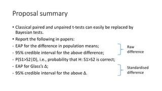
![Statistical models (classical and Bayesian)
Paired test
Classical paired t-test:
score differences obey
Bayesian: scores obey
a bivariate
normal
distribution
Unpaired (=Two-sample) test
S1’s scores obey
S2’s scores obey
Classical test: Welch’s t-test
Bayesian:
Stan code
[Toyoda15]](https://image.slidesharecdn.com/sigir2017bayesian-170808065151/85/sigir2017bayesian-30-320.jpg)
![Effect size (Glass’s Δ) [Okubo+12]
• In the context of classical significance testing, [Sakai14SIGIRforum] stresses
the importance of reporting sample effect sizes and confidence intervals
(CIs).
• Given your system S1 and a well-known baseline S2 (e.g. BM25), let’s
consider the diff between S1 and S2 standardised by an “ordinary”
standard deviation (i.e., that of the baseline):
• With classical tests, this can simply be estimated from the sample.
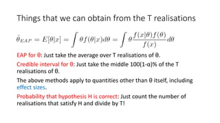
• With Bayesian tests, and EAP and a credible interval for Δ can easily be
obtained from the T realisations.
Unlike Cohen’s d/Hedges’ g, free from the
homoscedasticity assumption](https://image.slidesharecdn.com/sigir2017bayesian-170808065151/85/sigir2017bayesian-31-320.jpg)
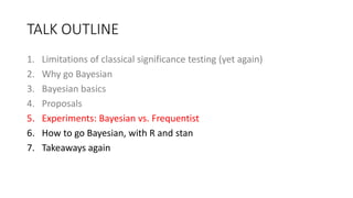
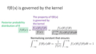
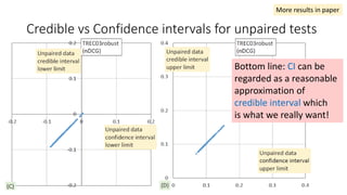
![EAP Δ vs sample Δ for paired tests
The classical sample Δ
probably underestimate
small effect sizes.
“the relevant question is asking which
method provides the richest, most
informative, and meaningful results for
any set of data. The answer is always
Bayesian estimation.” [Kruschke15]
More results in paper](https://image.slidesharecdn.com/sigir2017bayesian-170808065151/85/sigir2017bayesian-38-320.jpg)
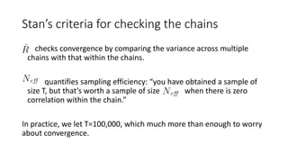
![EAP Δ vs sample Δ for paired tests – an anomalous result
• This measure from the TREC Temporal
Summarisation Track [Aslam+16] is like a
nugget-based F-measure over a timeline.
• The actual score distribution of this
measure is [0, 0.4021] rather than [0,1],
with very low standard deviations (and
hence very high effect sizes).
• The measure is not as well-understood as
the others and deserves an investigation.](https://image.slidesharecdn.com/sigir2017bayesian-170808065151/85/sigir2017bayesian-39-320.jpg)
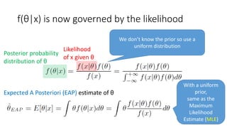
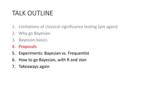
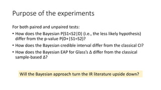
![EAP Δ vs sample Δ for unpaired tests
The classical sample Δ
probably underestimate
small effect sizes.
“the relevant question is asking which
method provides the richest, most
informative, and meaningful results for
any set of data. The answer is always
Bayesian estimation.” [Kruschke15]
same sample Δ from the paired test experiments](https://image.slidesharecdn.com/sigir2017bayesian-170808065151/85/sigir2017bayesian-42-320.jpg)
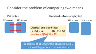
![EAP Δ vs sample Δ for unpaired tests – an anomalous result
• This measure from the TREC Temporal
Summarisation Track [Aslam+16] is like a
nugget-based F-measure over a timeline.
• The actual score distribution of this
measure is [0, 0.4021] rather than [0,1],
with very low standard deviations (and
hence very high effect sizes).
• The measure is not as well-understood as
the others and deserves an investigation.](https://image.slidesharecdn.com/sigir2017bayesian-170808065151/85/sigir2017bayesian-43-320.jpg)
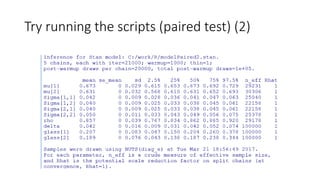
![Try running the scripts (paired test) (1)
Try this (BayesPaired-sample.R) on the R interface:
library(rstan)
scr <- "C:/work/R/modelPaired2.stan" #model written in Stan (see sample file)
par <- c( "mu", "Sigma", "rho", "delta", "glass" ) #mean, variances, correlation, delta, glass's delta
war <- 1000 #burn-in
ite <- 21000 #iteration including burn-in
see <- 1234 #seed
dig <- 3 #significant digits
cha <- 5 #chains (number of trials = (ite-war)*cha)
source( "C:/work/R/run1_vs_run2.paired.R" ) #per-topic scores (see sample file)
outfile <- "C:/work/R/run1_vs_run2.NUTS.paired.csv" #output files
data <- list( N=N, x=x ) #sample size and per-topic scores
fit <- stan( file=scr, model_name=scr, data=data, pars=par, verbose=F, seed=see, algorithm="NUTS", chains=cha, warmup=war, iter=ite, sample_file=outfile )
# compile stan file and execute sampling (HMC may be used instead of NUTs)
print( fit, pars=par, digits_summary=dig )
Five output csv files:
C:/work/R/run1_vs_run2.NUTS.paired_[1-5].csv](https://image.slidesharecdn.com/sigir2017bayesian-170808065151/85/sigir2017bayesian-47-320.jpg)
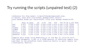
![Try running the scripts (unpaired test) (1)
Try this (BayesPaired-sample.R) on the R interface:
library(rstan)
scr <- "C:/work/R/modelUnpaired2.stan" #model written in Stan (see sample file)
par <- c( "mu1", "mu2", "sigma1", "sigma2", "delta", "glass" ) #means, s.d.'s, delta, glass's delta
war <- 1000 #burn-in
ite <- 21000 #iteration including burn-in
see <- 1234 #seed
dig <- 3 #significant digits
cha <- 5 #chains (number of trials = (ite-war)*cha)
source( "C:/work/R/run1_vs_run2.unpaired.R" ) #per-topic scores (see sample file)
outfile <- "C:/work/R/run1_vs_run2.NUTS.unpaired.csv" #output files
data <- list( N1=N1, N2=N2, x1=x1, x2=x2 ) #sample sizes and per-topic scores
fit <- stan( file=scr, model_name=scr, data=data, pars=par, verbose=F, seed=see, algorithm="NUTS", chains=cha, warmup=war, iter=ite, sample_file=outfile )
# compile stan file and execute sampling (HMC may be used instead of NUTs)
print( fit, pars=par, digits_summary=dig )
Five output csv files:
C:/work/R/run1_vs_run2.NUTS.unpaired_[1-5].csv](https://image.slidesharecdn.com/sigir2017bayesian-170808065151/85/sigir2017bayesian-50-320.jpg)
![References (1)
[Aslam+16] TREC 2015 Temporal Summarization Track, TREC 2015, 2016.
[Bayes1763] An Essay towards Solving a Problem in the Doctrine of Chances.
Philosophical Transactions of the Royal Society of London, 53, 1763.
[Carterette11] Model-based Inference about IR Systems. ICTIR 2011 (LNCS 6931).
[Carterette15] Bayesian Inference for Information Retrieval Evaluation, ACM ICTIR
2015.
[Cohen1990] Things I Have Learned (So Far). American Psychologist, 45(12), 1990.
[Fisher1970] Statistical Methods for Research Workers (14th Edition). Oliver & Boyd,
1970.
[Kruschke13] Bayesian Estimation Supersedes the t test. Journal of Experimental
Psychology: General, 142(2), 2013.
[Hoffman+14] The No-U-Turn Sampler: Adaptively Setting Path Lengths in
Hamiltonian Monte Carlo. Journal of Machine Learning Research, 15, 2014.](https://image.slidesharecdn.com/sigir2017bayesian-170808065151/85/sigir2017bayesian-56-320.jpg)
![References (2)
[Kruschke15] Doing Bayesian Data Analysis. Elsevier, 2015.
[Neal11] MCMC using Hamiltonian Dynamics. In: Handbook of Markov Chain
Monte Carlo, Chapman & Hall, 2015.
[Okubo+12] Psychological Statistics to Tell Your Story: Effect Size, Confidence
Interval, and Power. Keiso Shobo, 2012.
[Sakai14forum] Statistical Reform in Information Retrieval? SIGIR Forum 48(1), 2014.
[Toyoda15] Fundamentals of Bayesian Statistics: Practical Getting Started by
Hamiltonian Monte Carlo Method (in Japanese). Asakura Shoten, 2015.
[Wasserstein+16] The ASA’s Statement on P-values: Context, Process, and Purpose.
The American Statistician, 2016.
[Zhang+16] Bayesian Performance Comparison of Text Classifiers. ACM SIGIR 2016.
[Ziliak+08] The Cult of Statistical Significance: How the Standard Error Costs Us Jobs,
Justice, and Lives. The University of Michigan Press, 2008.](https://image.slidesharecdn.com/sigir2017bayesian-170808065151/85/sigir2017bayesian-57-320.jpg)

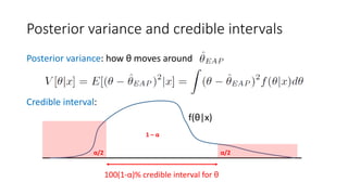
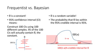
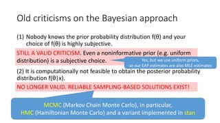
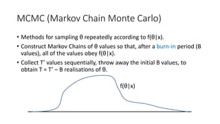
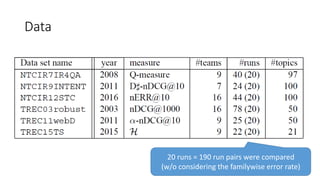
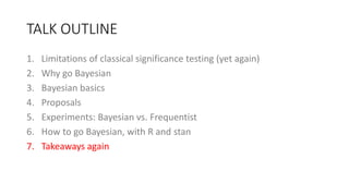
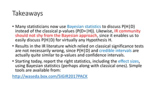
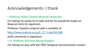
The document discusses limitations of classical significance testing and advantages of Bayesian statistics for information retrieval (IR) evaluation. It proposes that the IR community should adopt the Bayesian approach to directly discuss the probability that a hypothesis is true given observed data. Bayesian methods allow estimating this probability for any hypothesis, using tools like Markov chain Monte Carlo sampling and Hamiltonian Monte Carlo. The document recommends always reporting effect sizes alongside probabilities to provide full understanding of results.