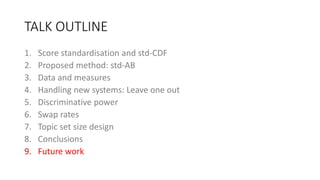
Download as PDF, PPTX

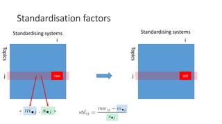
![Score standardisation [Webber+08]
standardised score for i-th system, j-th topic
j
i
raw
Topics
Systems
j
i
std
Topics
Systems
Subtract mean;
divide by standard deviation
How good is i compared to
“average” in standard
deviation units?
Standardising factors](https://image.slidesharecdn.com/ictir2016-160910034014/85/ictir2016-5-320.jpg)
![Standardised scores have the [-∞, ∞] range
and are not very convenient.
-2
-1
0
1
2
System 1System 2System 3System 4System 5
Topic 1 Topic 2
Transform them back into the [0,1] range!](https://image.slidesharecdn.com/ictir2016-160910034014/85/ictir2016-7-320.jpg)
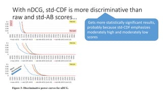
![std-CDF: use the cumulative density function of
the standard normal distribution [Webber+08]
0
0.2
0.4
0.6
0.8
1
0 0.1 0.2 0.3 0.4 0.5 0.6 0.7 0.8 0.9 1
TREC04
Each curve is
a topic, with
110 runs
represented
as dots
raw nDCG
std-CDF
nDCG](https://image.slidesharecdn.com/ictir2016-160910034014/85/ictir2016-8-320.jpg)

![std-AB with clipping, with the range [0,1]
Let B=0.5 (“average” system)
Let A=0.15 so that 89% of scores fall within [0.05, 0.95]
(Chebyshev’s inequality)
For EXTREMELY good/bad systems…
This formula with (A,B) is used in educational
research: A=100, B=500 for SAT, GRE [Lodico+10],
A=10, B=50 for Japanese hensachi “standard scores”.](https://image.slidesharecdn.com/ictir2016-160910034014/85/ictir2016-12-320.jpg)
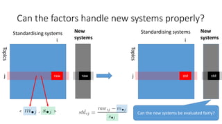
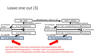
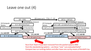
![Leave one out (1)
QR = {QRj} QR’(t) = {QR’j(t)}
(0) Leave out t, T’(t) = T – {t}
(1) Compute measure (1’) Compute measure
N × (M – L) matrix R QR’(t),T’(t) R QR’(t),{t}N × M matrix R QR,T
Runs from Team t have been removed from the pooled systems
– are these “new” runs evaluated fairly?
Compare two run rankings before and after leave one out
by means of Kendall’s tau.
original qrels
Evaluating M runs
using N topics
qrels with unique contributions from
Team t with L runs removed
L runsM - L runs
Zobel’s original method [Zobel98] removed one run at a time
but removing the entire team is more realistic [Voorhees02].](https://image.slidesharecdn.com/ictir2016-160910034014/85/ictir2016-20-320.jpg)
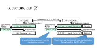
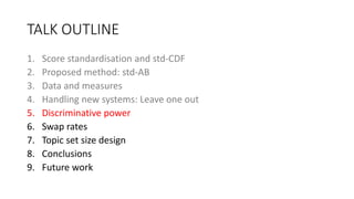
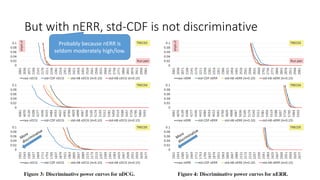
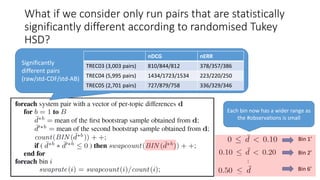
![Discriminative power
• Conduct a significance test for every system pair and plot the p-values
• Discriminative measures = those with small p-values
• [Sakai06SIGIR] used the bootstrap test for every system pair but using
k pairwise tests independently means that the familywise error rate
can amount to 1-(1-α) [Carterette12, Ellis10].
• [Sakai12WWW] used the randomised Tukey HSD test
[Carterette12][Sakai14PROMISE] instead to ensure that the
familywise error rate is bounded above by α.
k
We also use randomised Tukey HSD.](https://image.slidesharecdn.com/ictir2016-160910034014/85/ictir2016-26-320.jpg)
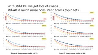
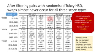
![Swap test
• System X > Y with topic set A. Does X > Y also hold with topic set B?
• [Voorhees09] splits 100 topics in half to form A and B, each with 50.
• [Sakai06SIGIR] showed that bootstrap samples (sampling with
replacement) can directly handle the original topic set size.
:
Bin 1
Bin 2
Bin 21](https://image.slidesharecdn.com/ictir2016-160910034014/85/ictir2016-30-320.jpg)
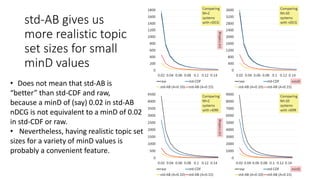
![Topic set size design [Sakai16IRJ,Sakai16ICTIRtutorial]
To determine the topic set size n for a new test collection to be built,
Sakai’s Excel tool based on one-way ANOVA power analysis takes as input:
α: Type I error probability
β: Type II error probability (power = 1 – β)
M: number of systems to be compared
minD: minimum detectable range
= minimum diff between the best and worst systems for which you want
to guarantee (1-β)% power
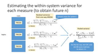
: estimate of the within-system variance (typically obtained from a
pilot topic-by-run matrix](https://image.slidesharecdn.com/ictir2016-160910034014/85/ictir2016-35-320.jpg)
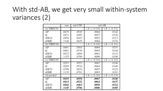
![With std-AB, we get very small within-system
variances (1)
The initial estimate of n with the one-way ANOVA topic set size design
is given by [Nagata03]
where,
for (α, β)=(0.05, 0.20), λ ≒
So n will be small if is small.
With std-AB, is indeed small because A is small (e.g. 0.15) and it can
be shown that
Noncentrality parameter of a noncentral
chi-square distribution](https://image.slidesharecdn.com/ictir2016-160910034014/85/ictir2016-37-320.jpg)
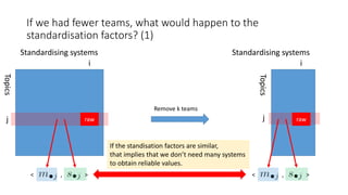
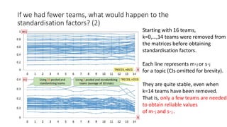
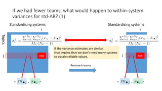
![If we had fewer teams, what would happen to within-system
variances for std-AB? (2)
Each k had 10 trials so 95% CIs of
the variance estimates are shown.
The variance estimates are also
stable even if we remove a lot of
teams. That is, only a few teams are
needed to obtain reliable variance
estimates for topic set size design.
Using std-AB with topic set size
design also means that we can
handle unnormalised measures
without any problems [Sakai16AIRS].](https://image.slidesharecdn.com/ictir2016-160910034014/85/ictir2016-43-320.jpg)


![Selected references (1)
[Carterette12] Carterette: Multiple testing in statistical analysis of
systems-based information retrieval experiments, ACM TOIS 30(1),
2012.
[Ellis10] Ellis: The essential guide to effect sizes, Cambridge, 2010.
[Lodico+10] Lodico, Spaulding, Voegtle: Methods in educational
research, Jossey-Bass, 2010.](https://image.slidesharecdn.com/ictir2016-160910034014/85/ictir2016-57-320.jpg)
![Selected references (2)
[Sakai06SIGIR] Sakai: Evaluating evaluation metrics based on the bootstrap, ACM
SIGIR 2006.
[Sakai12WWW] Sakai: Evaluation with Informational and Navigational Intents,
WWW 2012.
[Sakai14PROMISE] Sakai: Metrics, statistics, tests, PROMISE Winter School 2013
(LNCS 8173).
[Sakai16IRJ] Sakai: Topic set size design, Information Retrieval Journal 19(3), 2016.
http://link.springer.com/content/pdf/10.1007%2Fs10791-015-9273-z.pdf
[Sakai16ICTIRtutorial] Sakai: Topic set size design and power analysis in practice,
ICTIR 2016 Tutorial.
http://www.slideshare.net/TetsuyaSakai/ictir2016tutorial-65845256
[Sakai16AIRS] Sakai: The Effect of Score Standardisation on Topic Set Size Design,
AIRS 2016, to appear.](https://image.slidesharecdn.com/ictir2016-160910034014/85/ictir2016-58-320.jpg)
![Selected references (3)
[Voorhees02] Voorhees: The philosophy of information retrieval
evaluation, CLEF 2001.
[Voorhees09] Voorhees: Topic set size redux, ACM SIGIR 2009.
[Webber+08] Webber, Moffat, Zobel: Score standardisation for inter-
collection comparison of retrieval systems, ACM SIGIR 2008.
[Zobel98] Zobel: How reliable are the results of large-scale information
retrieval experiments? ACM SIGIR 1998.](https://image.slidesharecdn.com/ictir2016-160910034014/85/ictir2016-59-320.jpg)

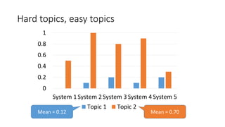
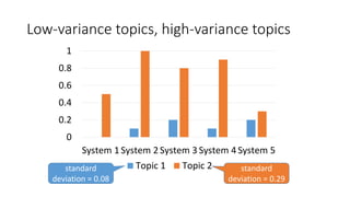
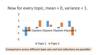
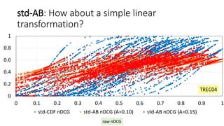
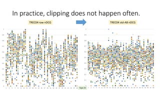
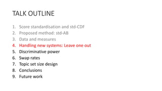
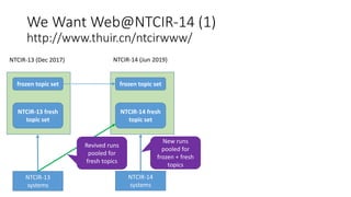
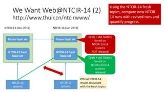
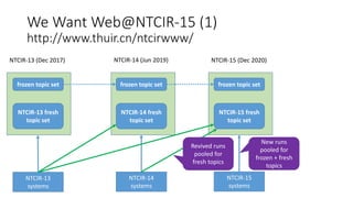
The document describes a simple and effective approach to score standardization called std-AB. It begins by discussing existing standardization methods like std-CDF and their limitations. It then proposes the std-AB method, which linearly transforms raw scores to have a range of 0 to 1. The document evaluates std-AB using several IR test collections and measures like nDCG and nERR. It finds that std-AB performs comparably to std-CDF in terms of ranking systems, handles new systems fairly in a leave-one-out test, and has fewer swaps between topic sets than std-CDF. The document concludes std-AB is a simple and effective alternative to existing standardization methods.