This document provides an overview of hypothesis testing basics:
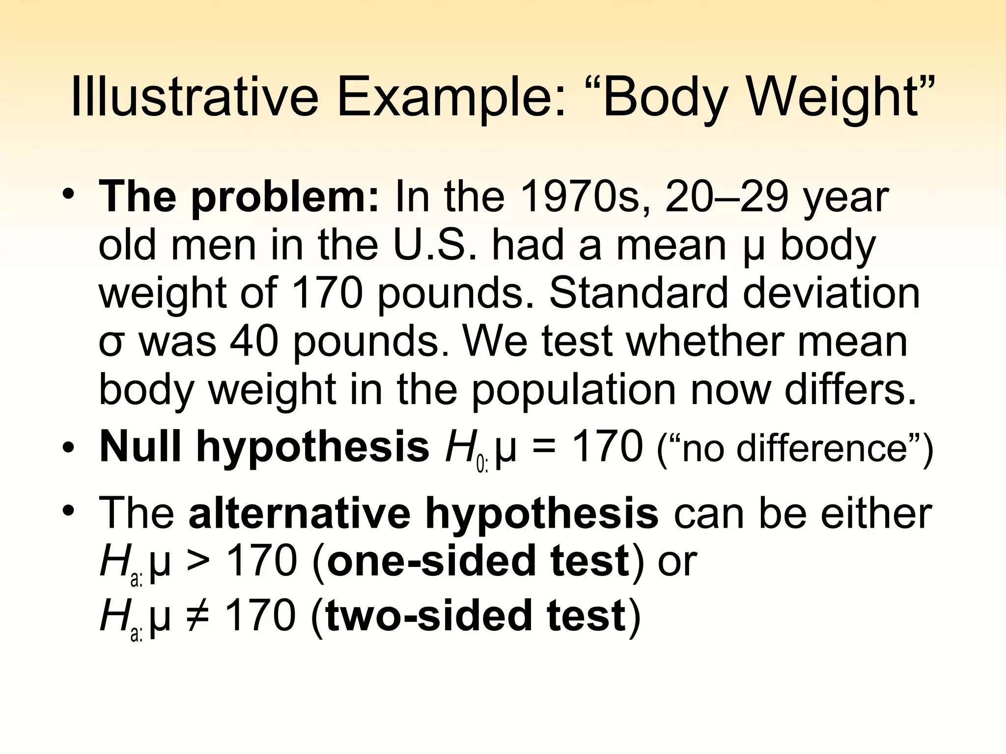
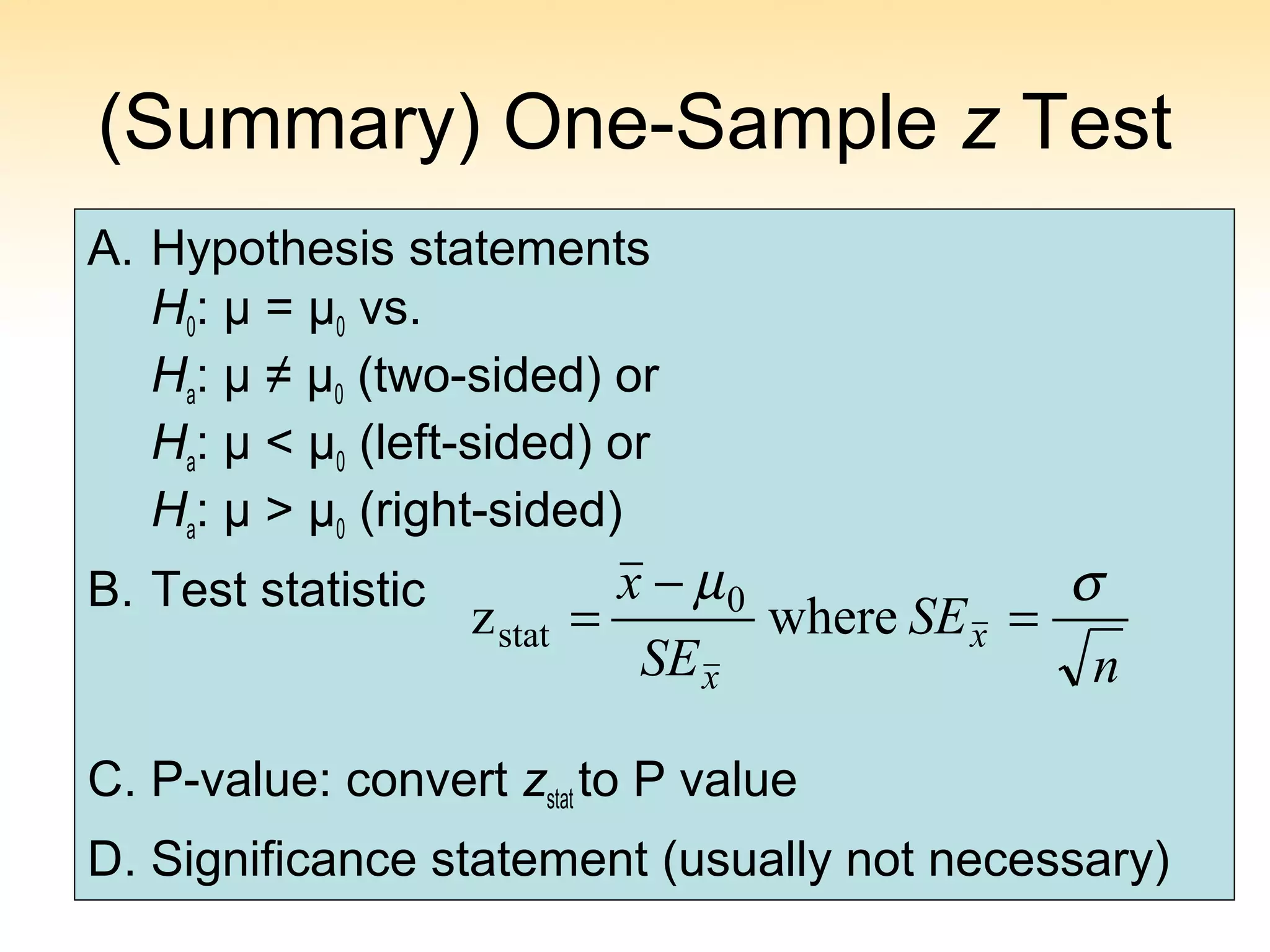
A) Hypothesis testing involves stating a null hypothesis (H0) and alternative hypothesis (Ha) based on a research question. H0 assumes no effect or difference, while Ha claims an effect.
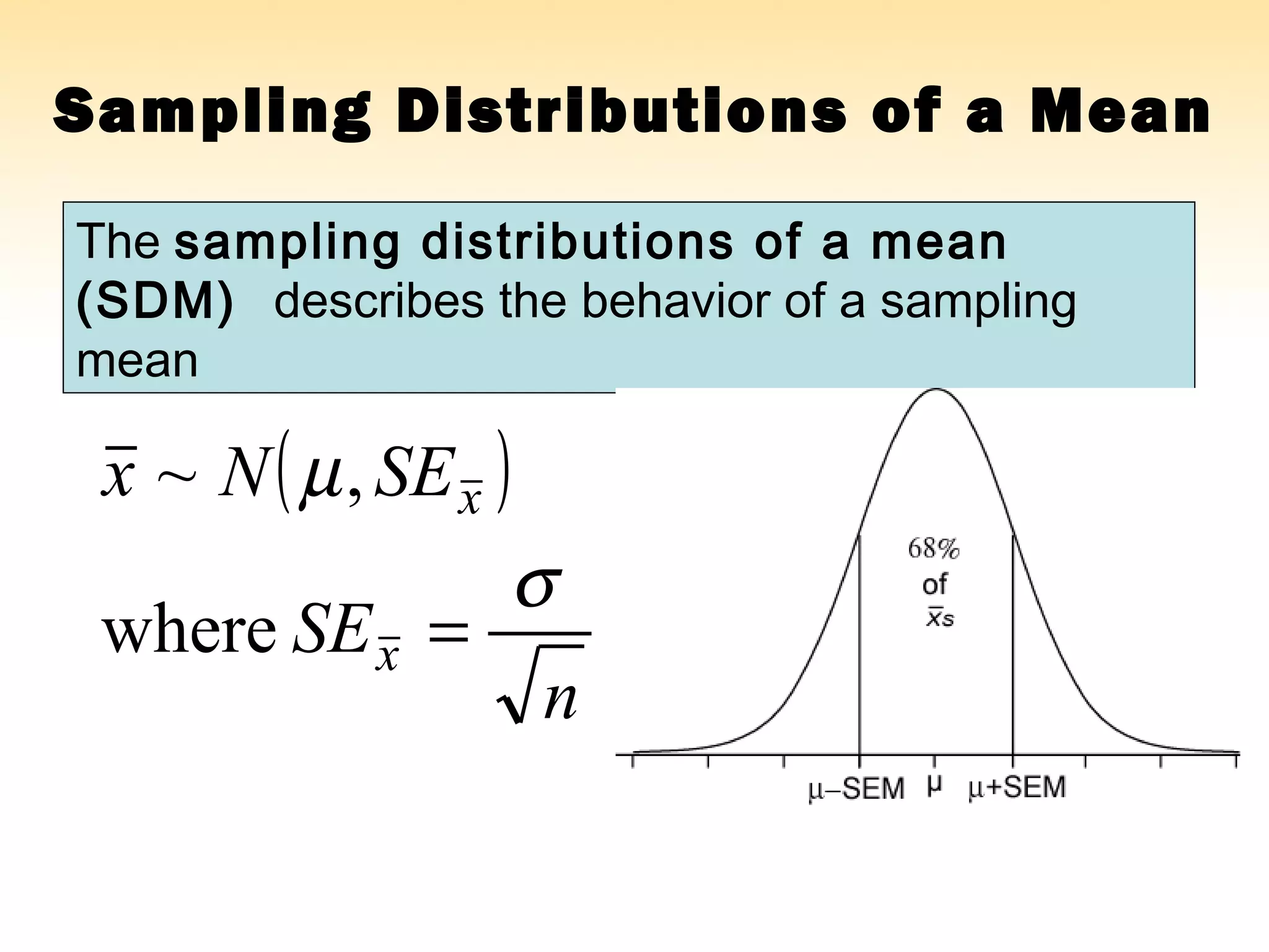
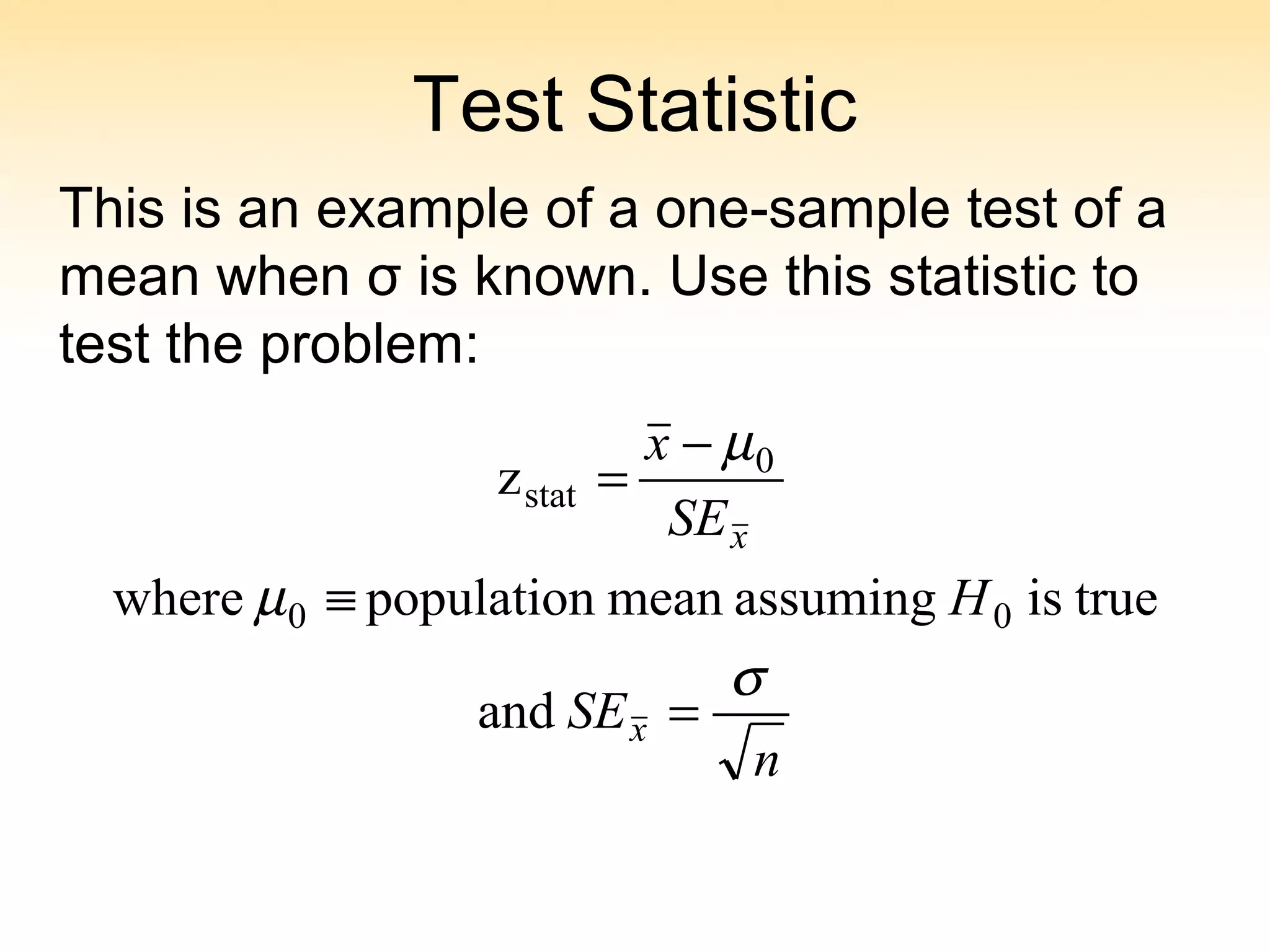
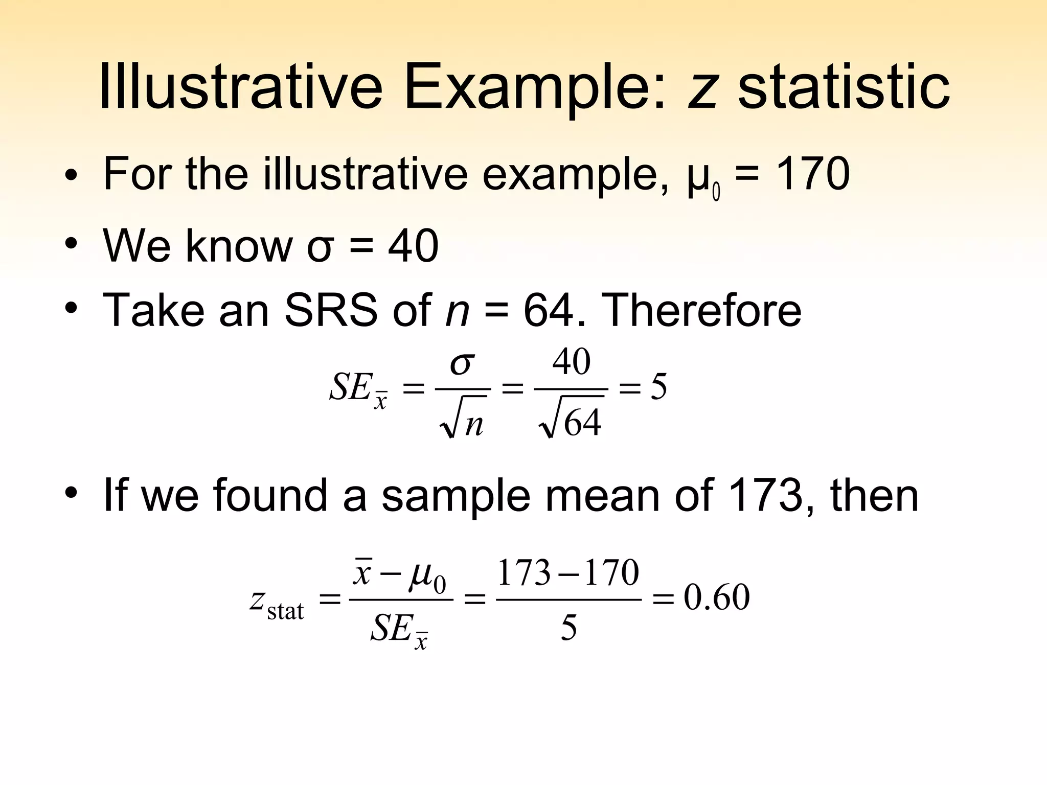
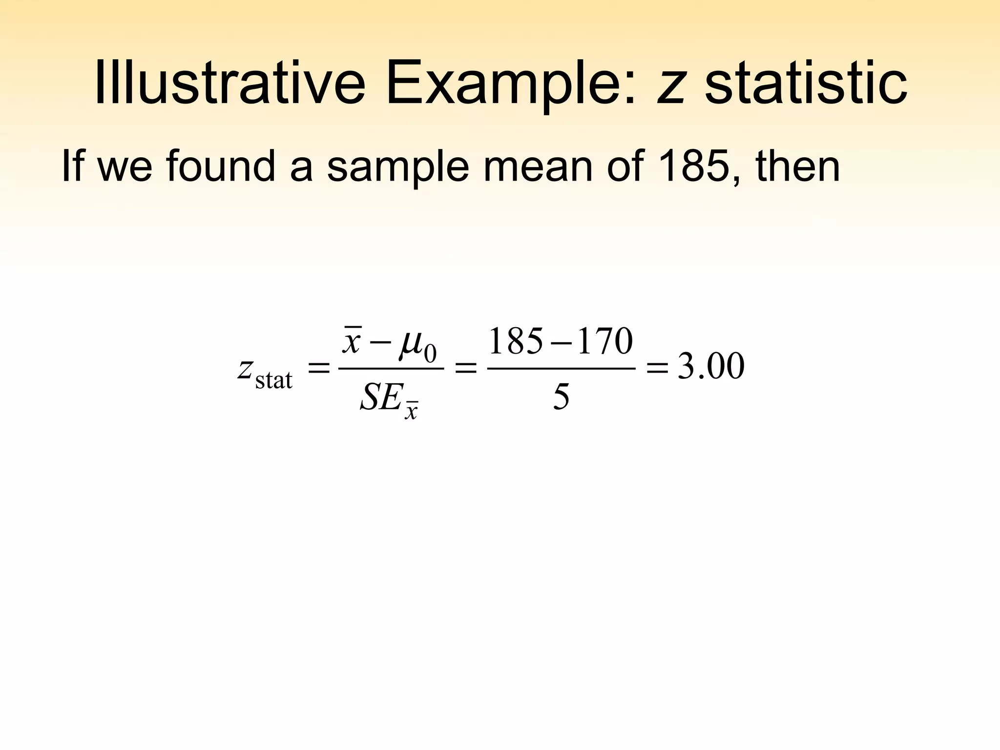
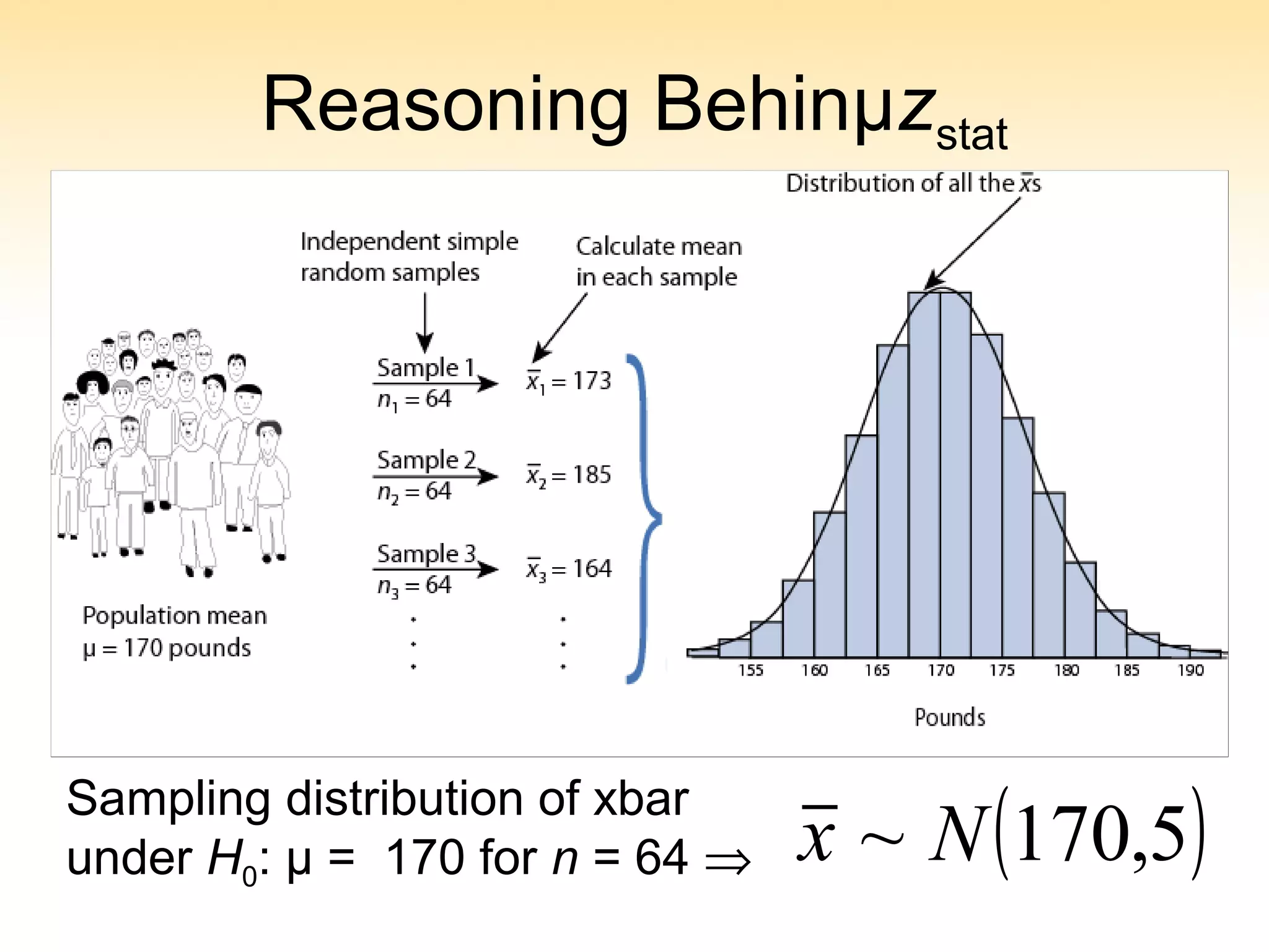
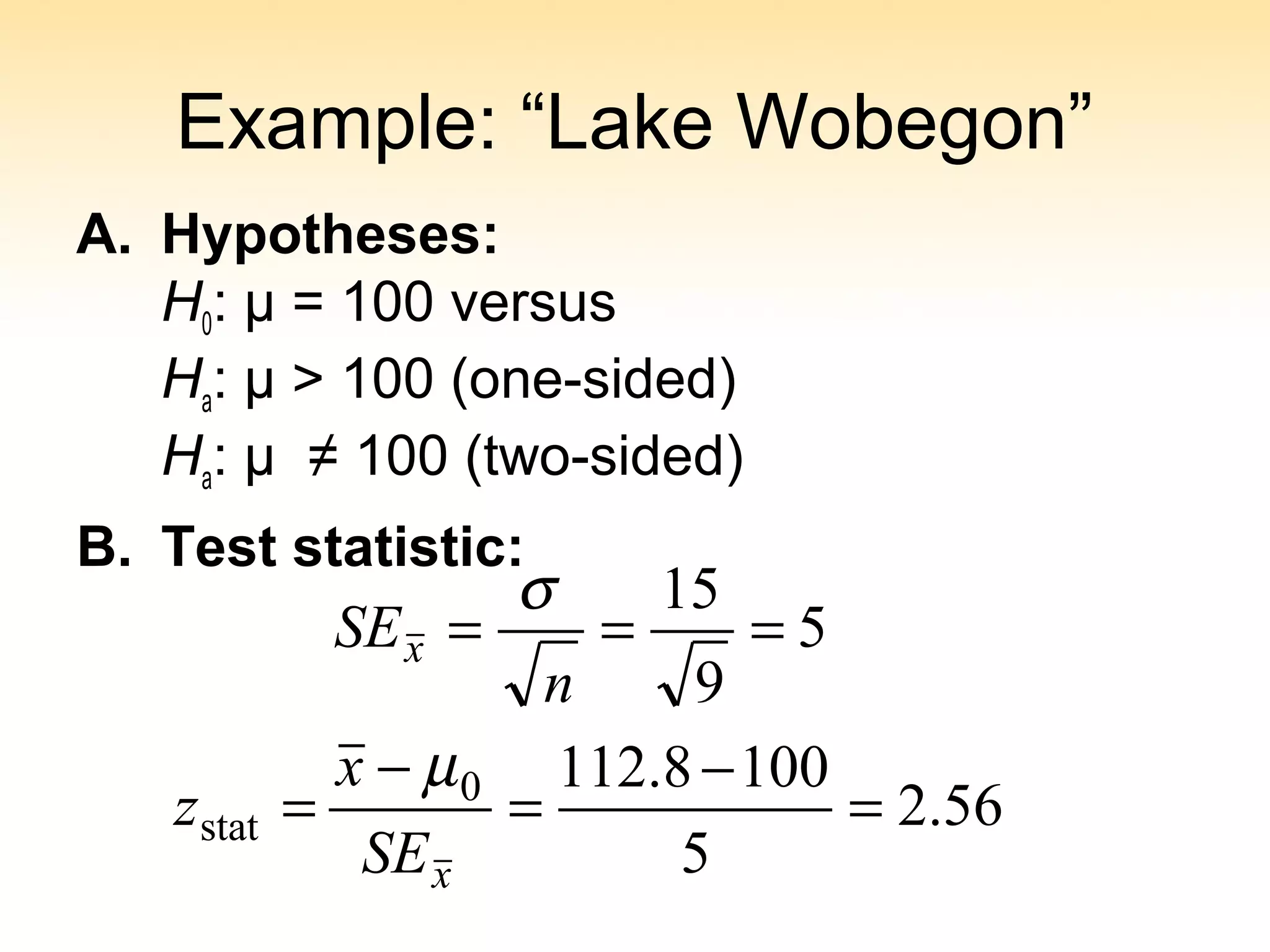
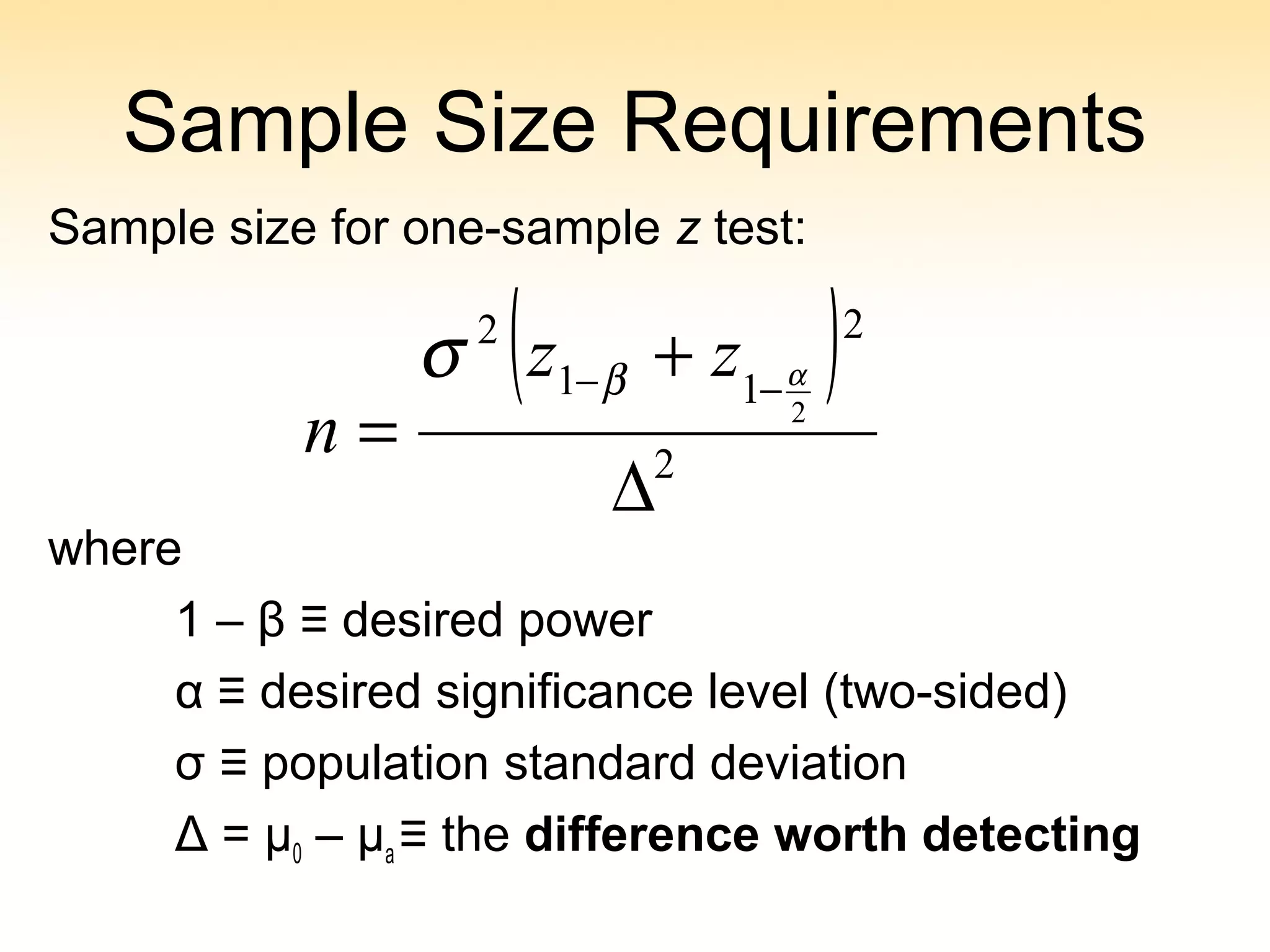
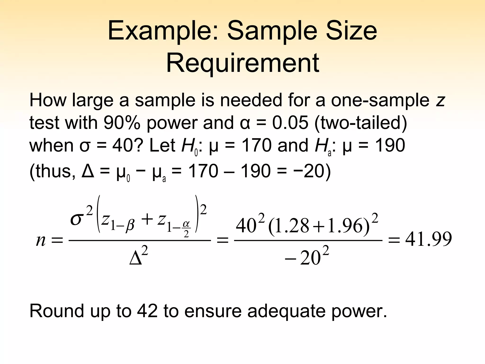
B) A test statistic is calculated from sample data and compared to a theoretical distribution to evaluate H0. For a one-sample z-test with known standard deviation, the test statistic is a z-score.
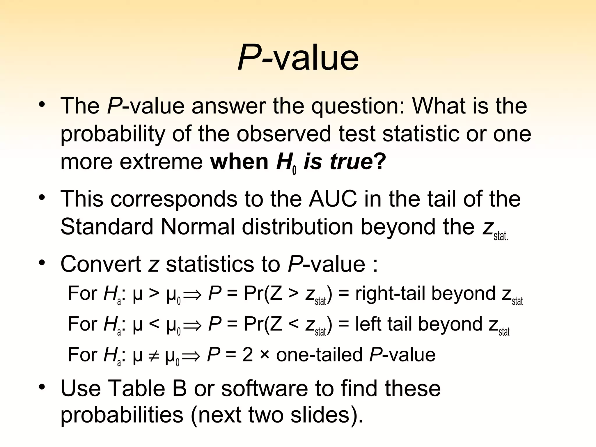
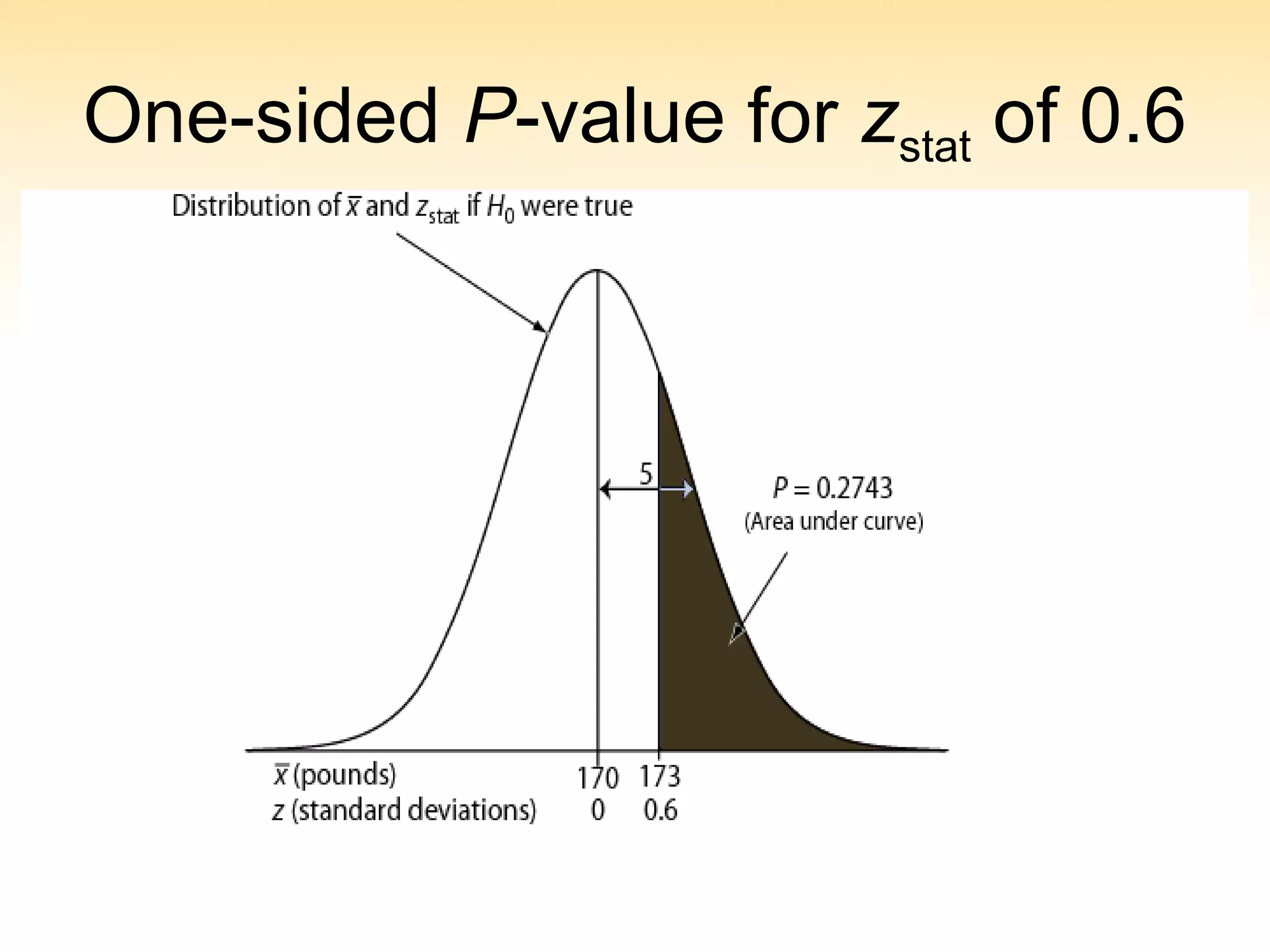
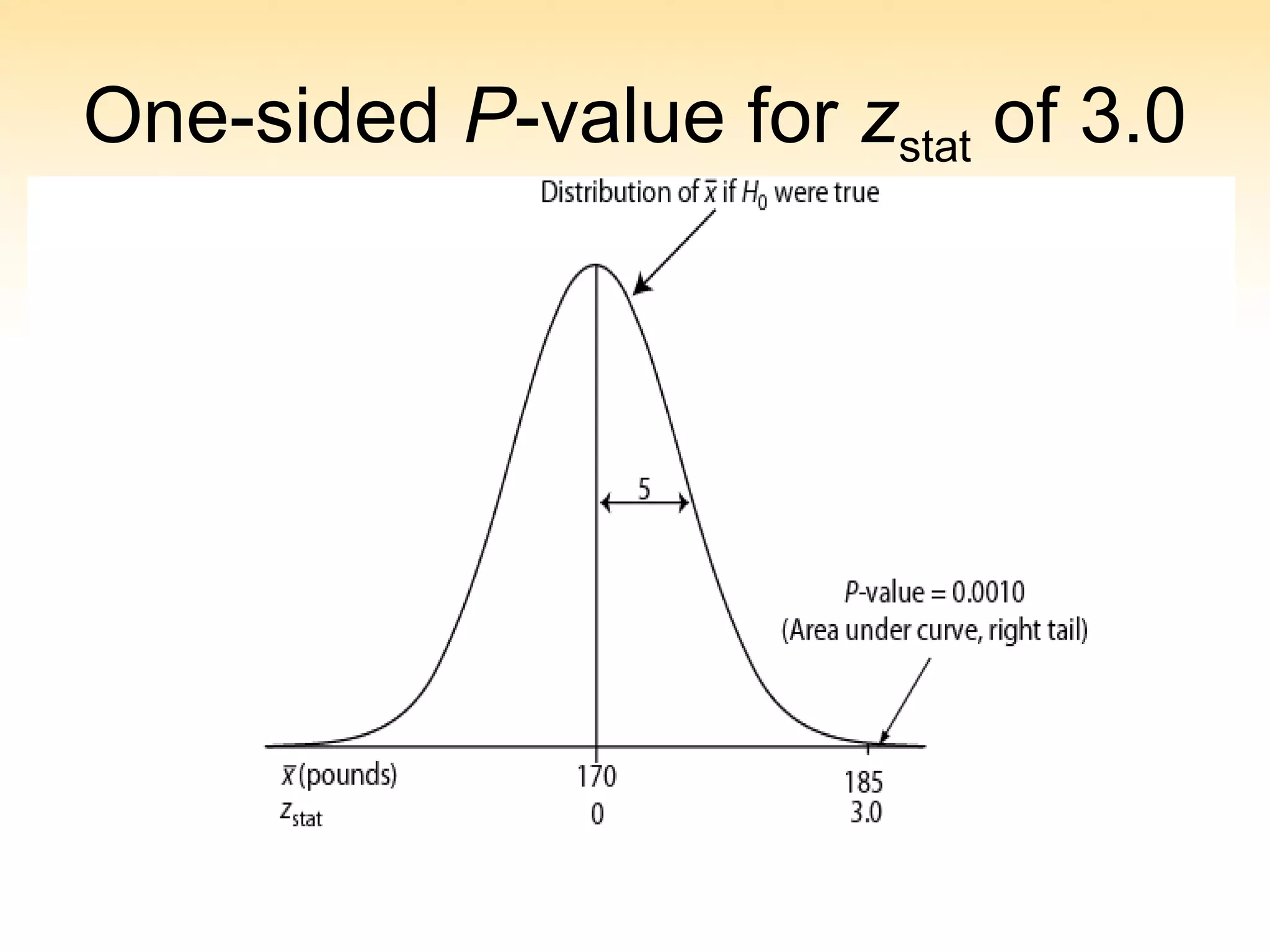
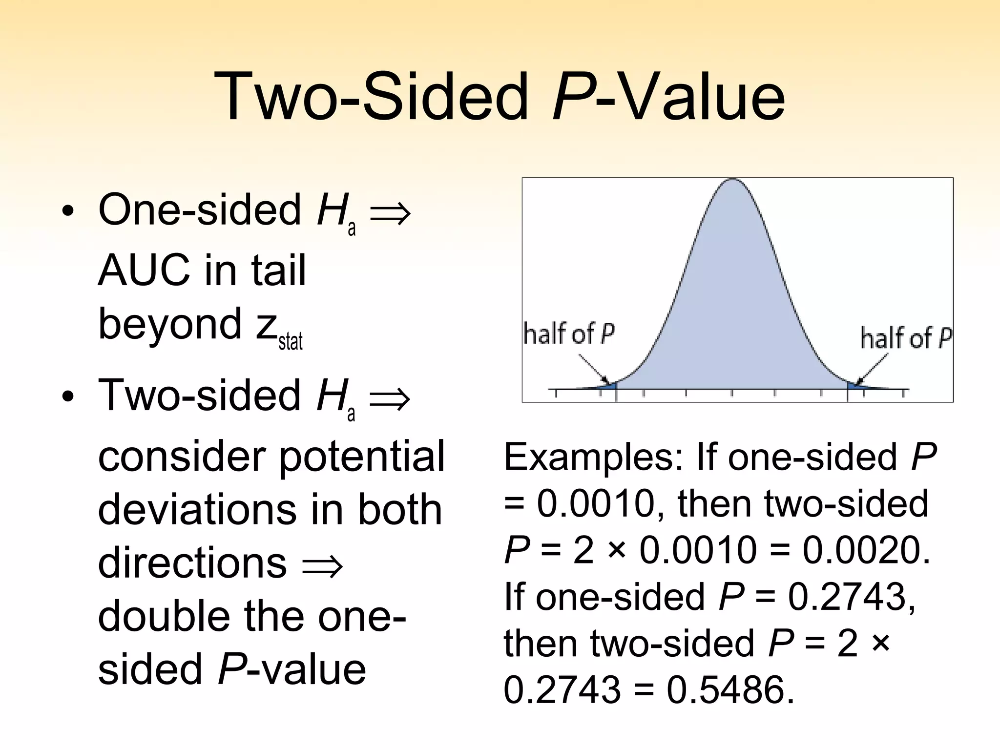
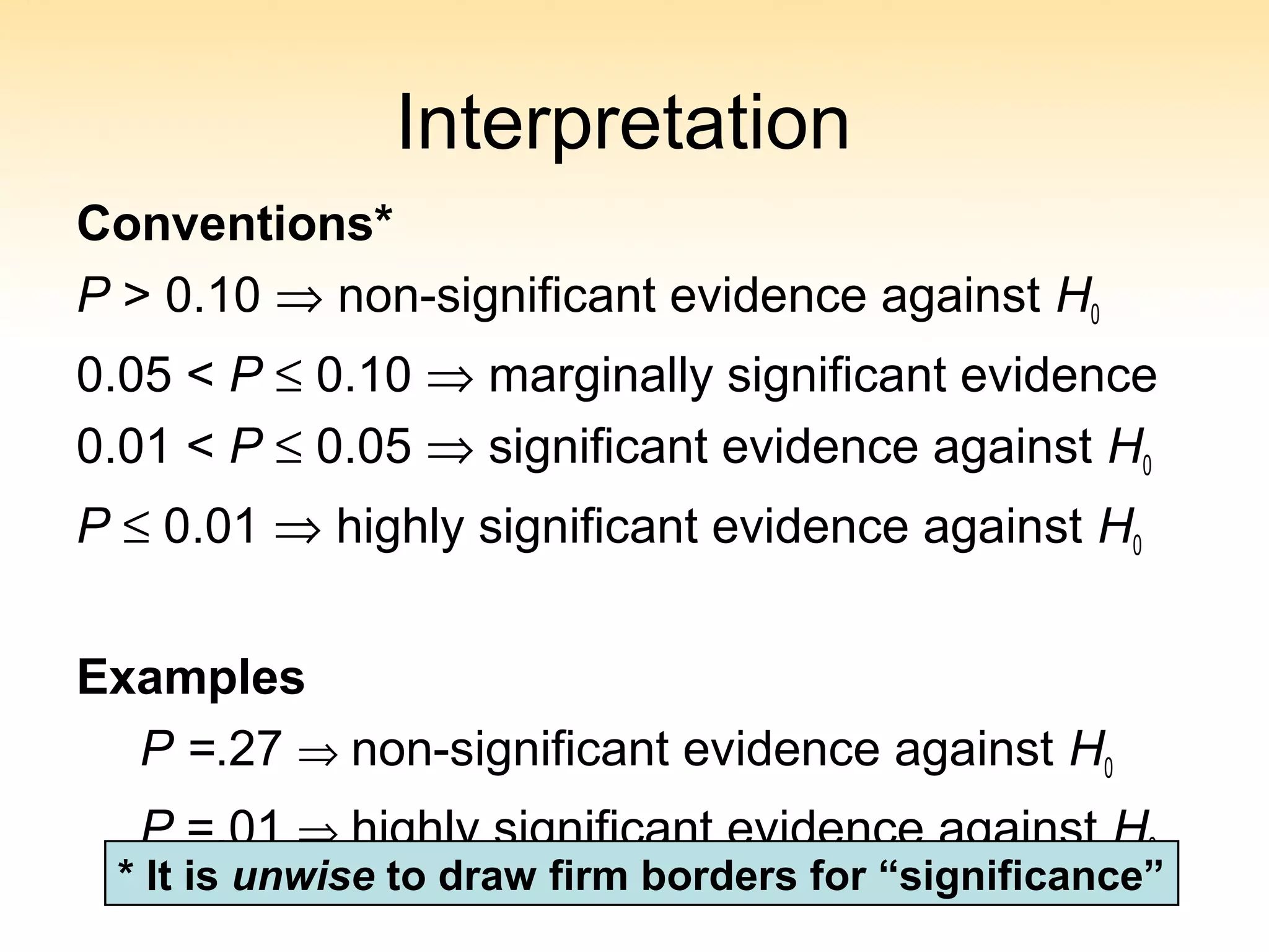
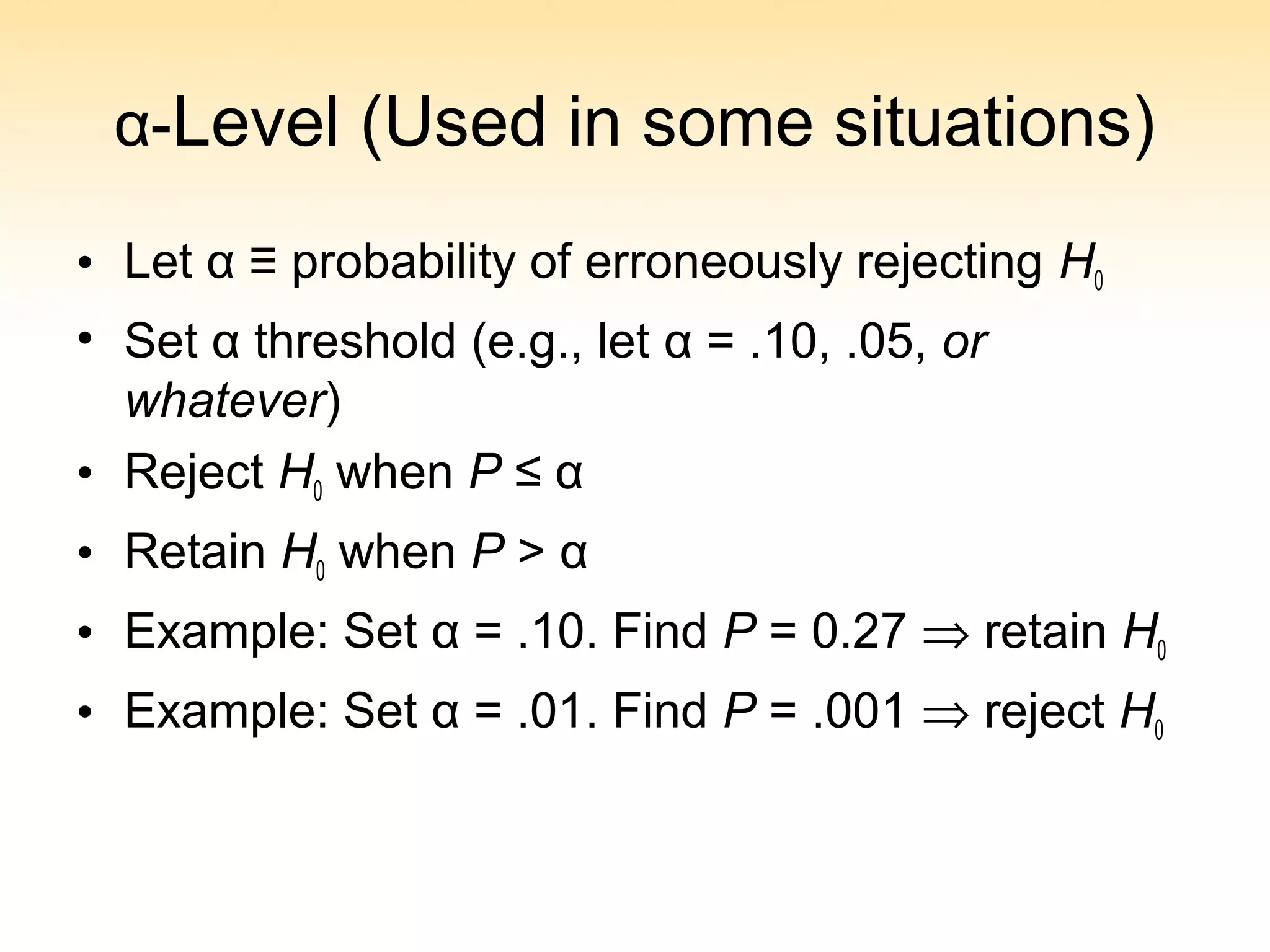
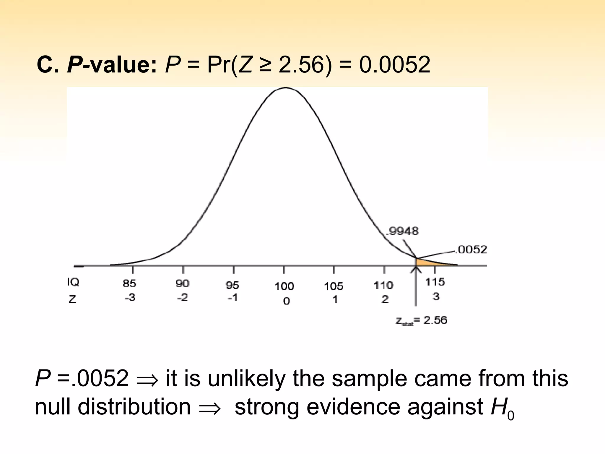
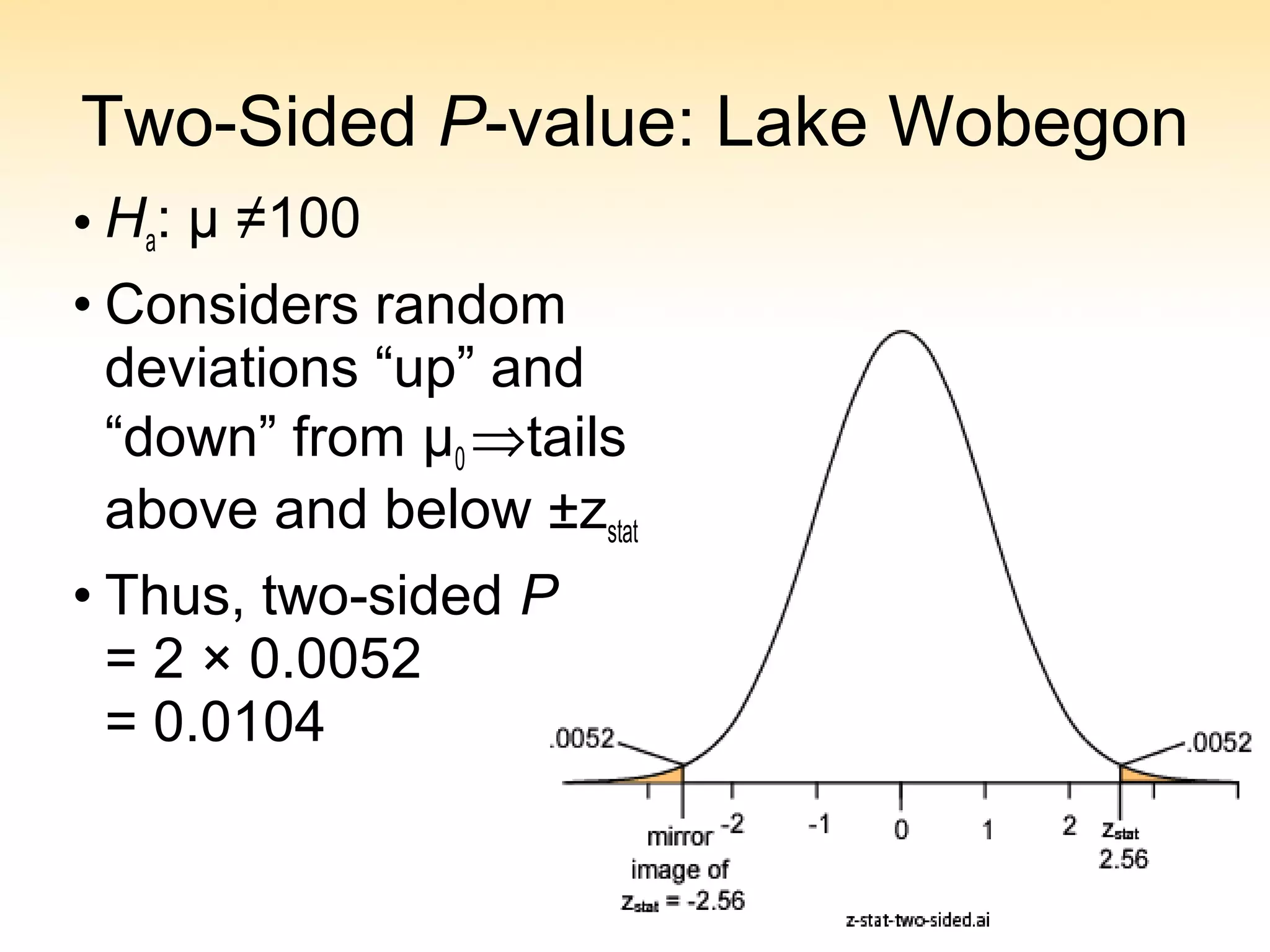
C) The p-value represents the probability of observing the test statistic or a more extreme value if H0 is true. Small p-values provide evidence against H0. Conventionally, p ≤ 0.05 is considered significant
![Basics of Hypothesis TestingBasics of Hypothesis Testing
By Prof Handley Mpoki MafwengaBy Prof Handley Mpoki Mafwenga
Ph.D, MSc, MBA, LLM, PGDTM, ADTM, LLB, FCTA(UK)Ph.D, MSc, MBA, LLM, PGDTM, ADTM, LLB, FCTA(UK)
Macro-fiscal Policy, Advocacy and Tax Expert [Gov-Macro-fiscal Policy, Advocacy and Tax Expert [Gov-
URT]URT]](https://image.slidesharecdn.com/f9365225-fa22-4e61-a12f-a46a02b06616-161229182557/75/Basic-of-Hypothesis-Testing-TEKU-QM-1-2048.jpg)