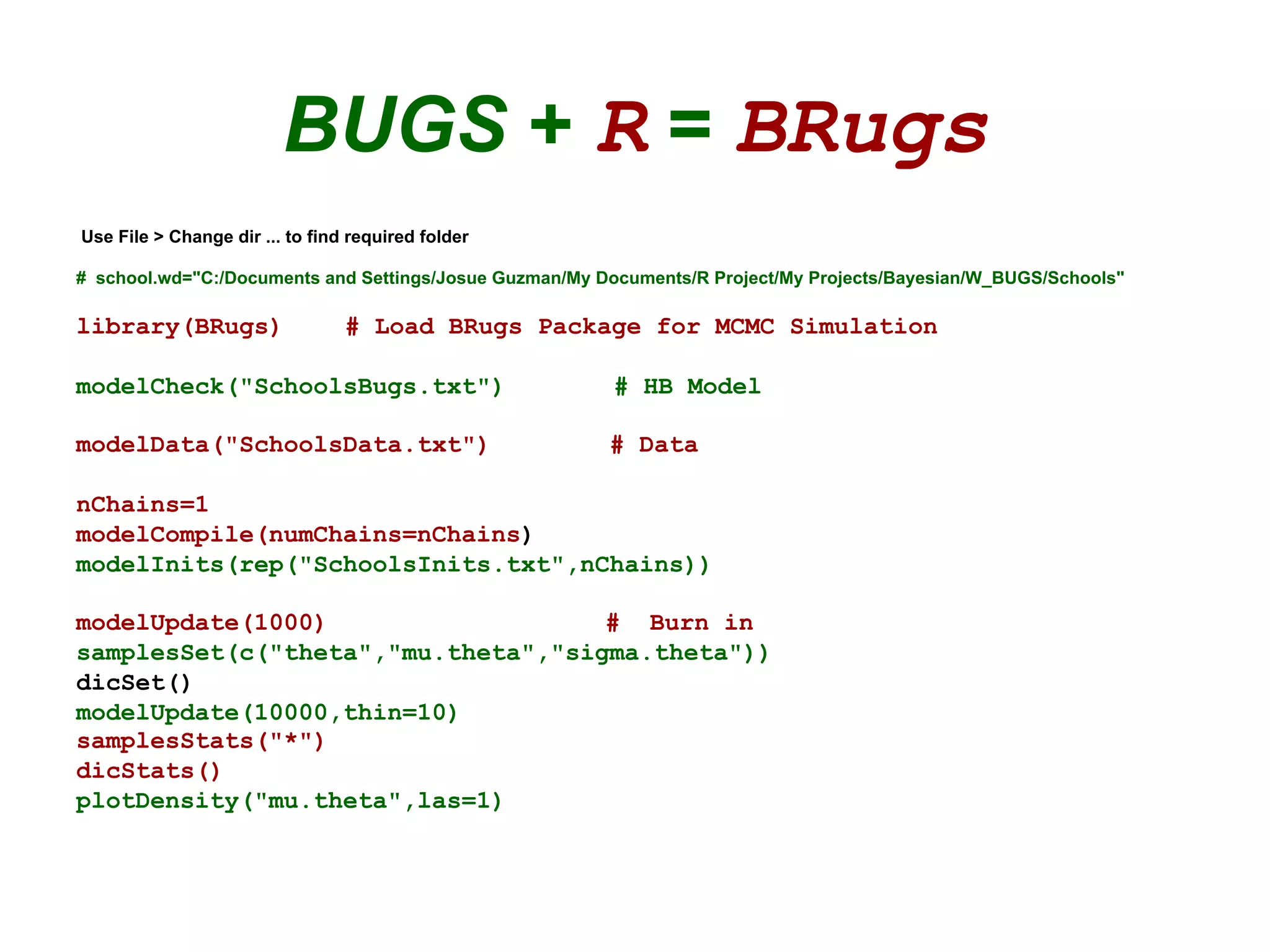
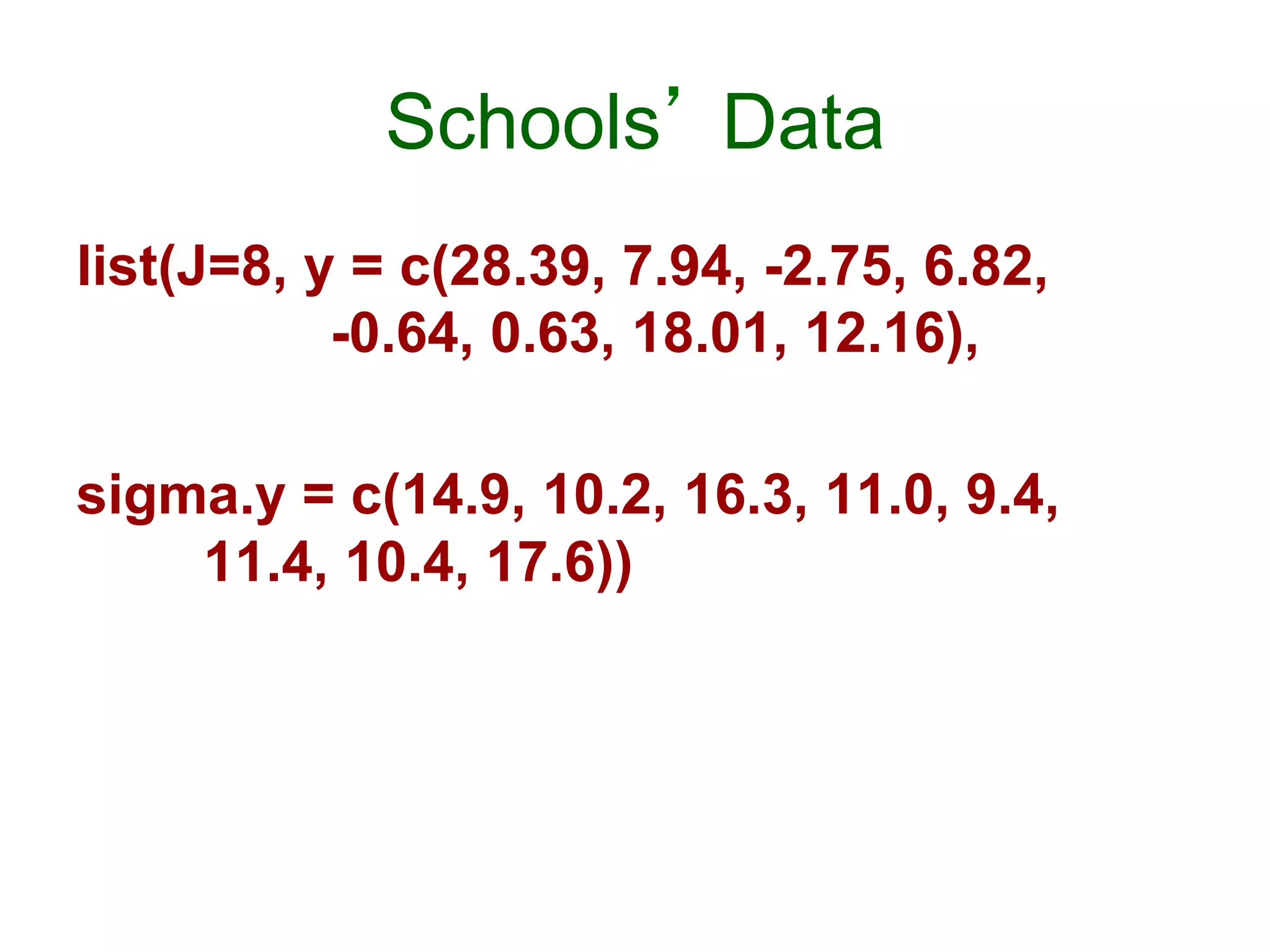
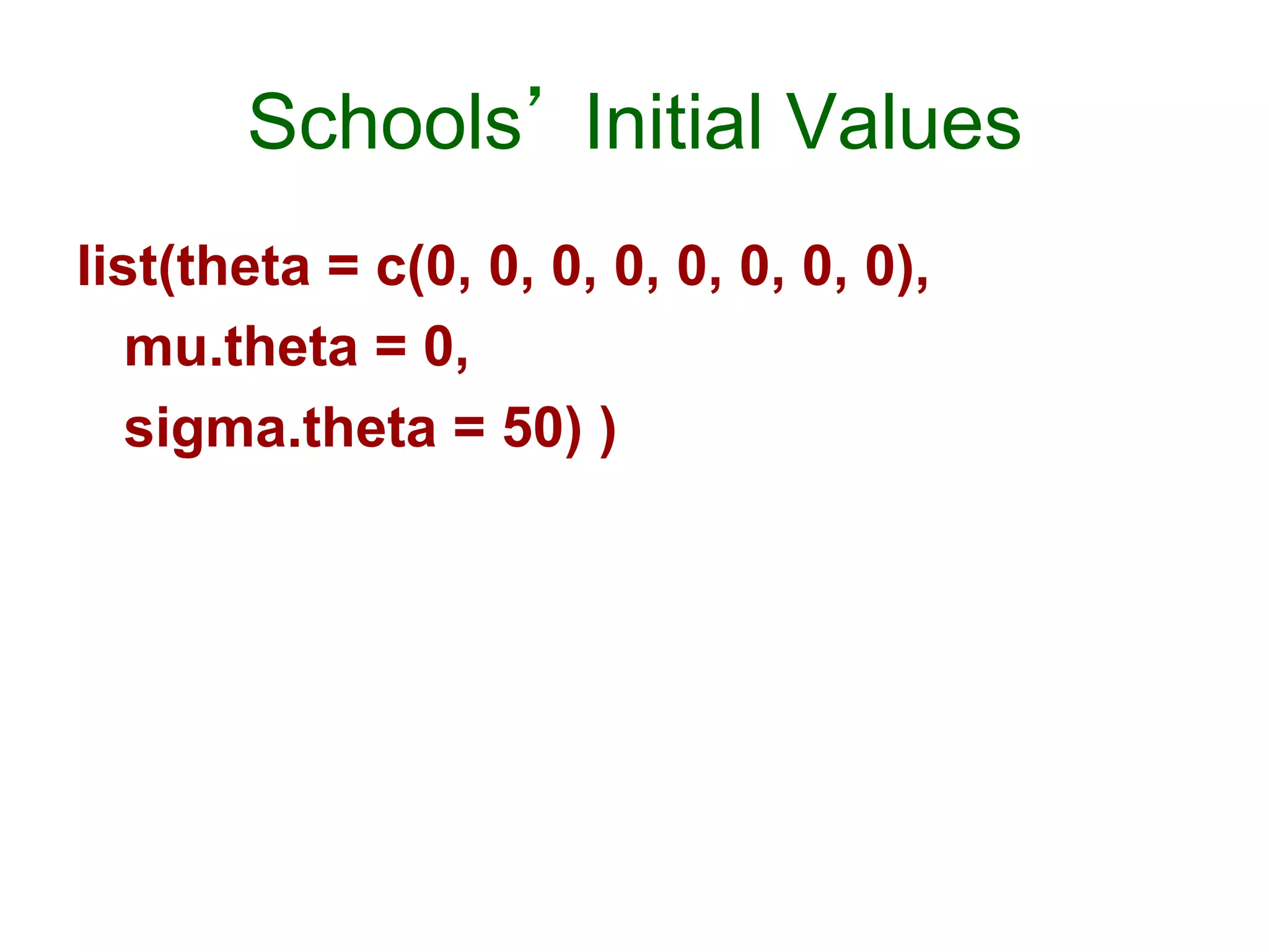
Download as PDF, PPTX
![Bayesian [Laplacean] Methods
• 1763 – Bayes’ article on inverse probability
• Laplace extended Bayesian ideas in different
scientific areas in Théorie Analytique des
Probabilités [1812]
• Laplace & Gauss used the inverse method
• 1st three quarters of 20th Century dominated by
frequentist methods [Fisher, Neyman, et al.]
• Last quarter of 20th Century – resurgence of
Bayesian methods [computational advances]
• 21st Century – Bayesian Century [Lindley]](https://image.slidesharecdn.com/bayesianstatisticsintrousingr-130906103849-/75/Bayesian-statistics-intro-using-r-6-2048.jpg)


![Community of Priors
• Expressing a range of reasonable opinions
• Reference – represents minimal prior
information [JM Bernardo, U of V]
• Expertise – formalizes opinion of
well-informed experts
• Skeptical – downgrades superiority of
new treatment
• Enthusiastic – counterbalance of skeptical](https://image.slidesharecdn.com/bayesianstatisticsintrousingr-130906103849-/75/Bayesian-statistics-intro-using-r-14-2048.jpg)
![Likelihood Function
P(data | θ)
• Represents the weight of evidence from the
experiment about θ
• It states what the experiment says about the
measure of interest [ LJ Savage, 1962 ]
• It is the probability of getting certain result,
conditioning on the model
• Prior is dominated by the likelihood as the
amount of data increases:
– Two investigators with different prior opinions
could reach a consensus after the results of an
experiment](https://image.slidesharecdn.com/bayesianstatisticsintrousingr-130906103849-/75/Bayesian-statistics-intro-using-r-15-2048.jpg)
![Example
• EXP 1: In a study of a
fixed sample of 20
students, 12 of them
respond positively to
the method [Binomial
distribution]
• Likelihood is
proportional to
θ12 (1 – θ)8
• EXP 2: Students are
entered into a study
until 12 of them
respond positively to
the method [Negative-
Binomial distribution]
• Likelihood at n = 20 is
proportional to
θ12 (1 – θ)8](https://image.slidesharecdn.com/bayesianstatisticsintrousingr-130906103849-/75/Bayesian-statistics-intro-using-r-18-2048.jpg)

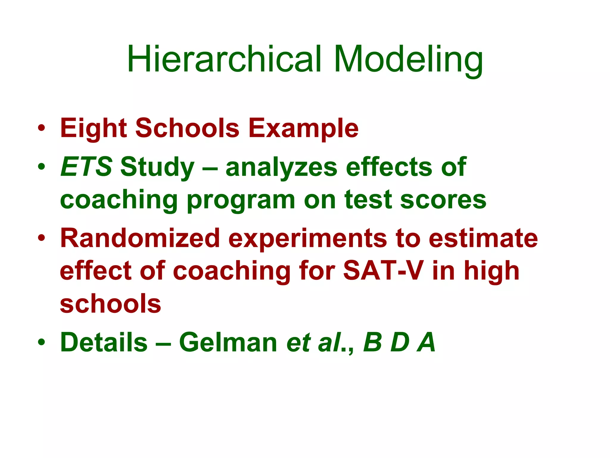
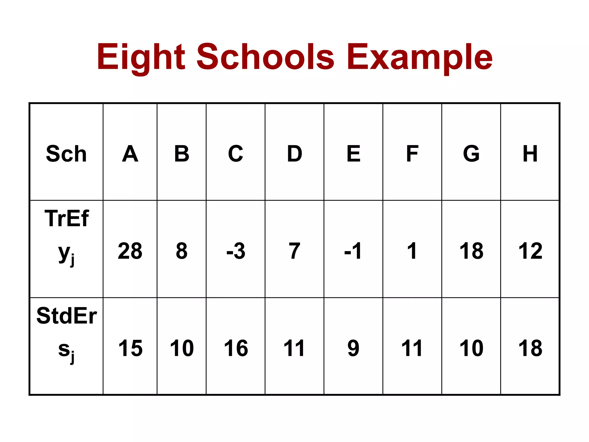
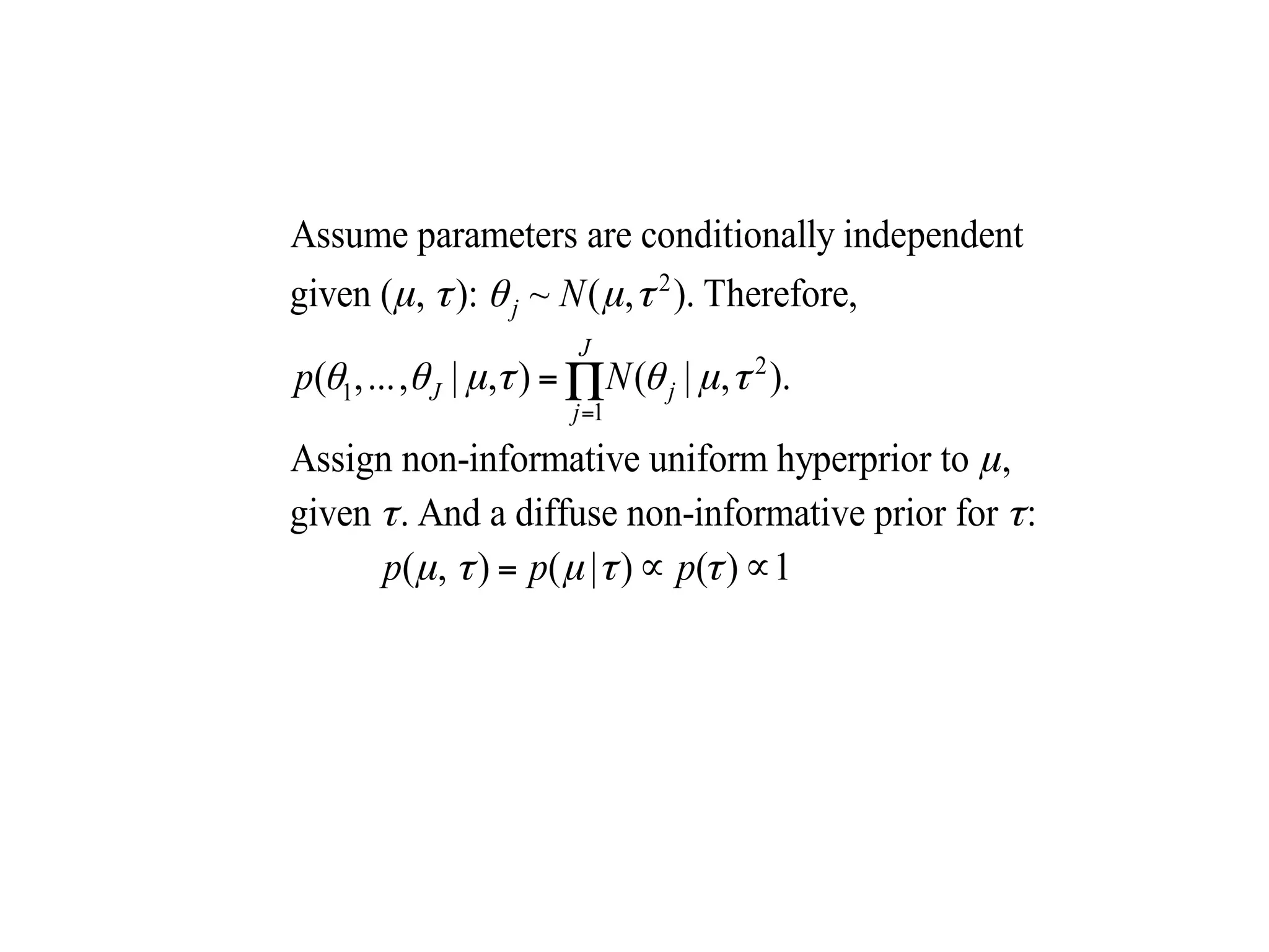
![Hierarchical Modeling
• θj ~ Normal(µ, σ) [Effect in School j]
• Uniform hyper–prior for µ, given σ; and
diffuse prior for σ:
Pr(µ, σ) = Pr(µ | σ) x Pr(σ) α 1
• Pr(µ, σ, θj | y ) = Pr(µ | σ) x p(σ) x
Π1:J [ θj | µ, σ] x Pr(y)](https://image.slidesharecdn.com/bayesianstatisticsintrousingr-130906103849-/75/Bayesian-statistics-intro-using-r-45-2048.jpg)

![Schools’ Model
model {
for (j in 1:J)
{
y[j] ~ dnorm (theta[j], tau.y[j])
theta[j] ~ dnorm (mu.theta, tau.theta)
tau.y[j] <- pow(sigma.y[j], -2)
}
mu.theta ~ dnorm (0.0, 1.0E-6)
tau.theta <- pow(sigma.theta, -2)
sigma.theta ~ dunif (0, 1000)
}](https://image.slidesharecdn.com/bayesianstatisticsintrousingr-130906103849-/75/Bayesian-statistics-intro-using-r-50-2048.jpg)
![BRugs Schools’ Results
samplesStats("*")
mean sd MCerror 2.5pc median 97.5pc start sample
mu.theta 8.147 5.28 0.081 -2.20 8.145 18.75 1001 10000
sigma.theta 6.502 5.79 0.100 0.20 5.107 21.23 1001 10000
theta[1] 11.490 8.28 0.098 -2.34 10.470 31.23 1001 10000
theta[2] 8.043 6.41 0.091 -4.86 8.064 21.05 1001 10000
theta[3] 6.472 7.82 0.103 -10.76 6.891 21.01 1001 10000
theta[4] 7.822 6.68 0.079 -5.84 7.778 21.18 1001 10000
theta[5] 5.638 6.45 0.091 -8.51 6.029 17.15 1001 10000
theta[6] 6.290 6.87 0.087 -8.89 6.660 18.89 1001 10000
theta[7] 10.730 6.79 0.088 -1.35 10.210 25.77 1001 10000
theta[8] 8.565 7.87 0.102 -7.17 8.373 25.32 1001 10000](https://image.slidesharecdn.com/bayesianstatisticsintrousingr-130906103849-/75/Bayesian-statistics-intro-using-r-53-2048.jpg)
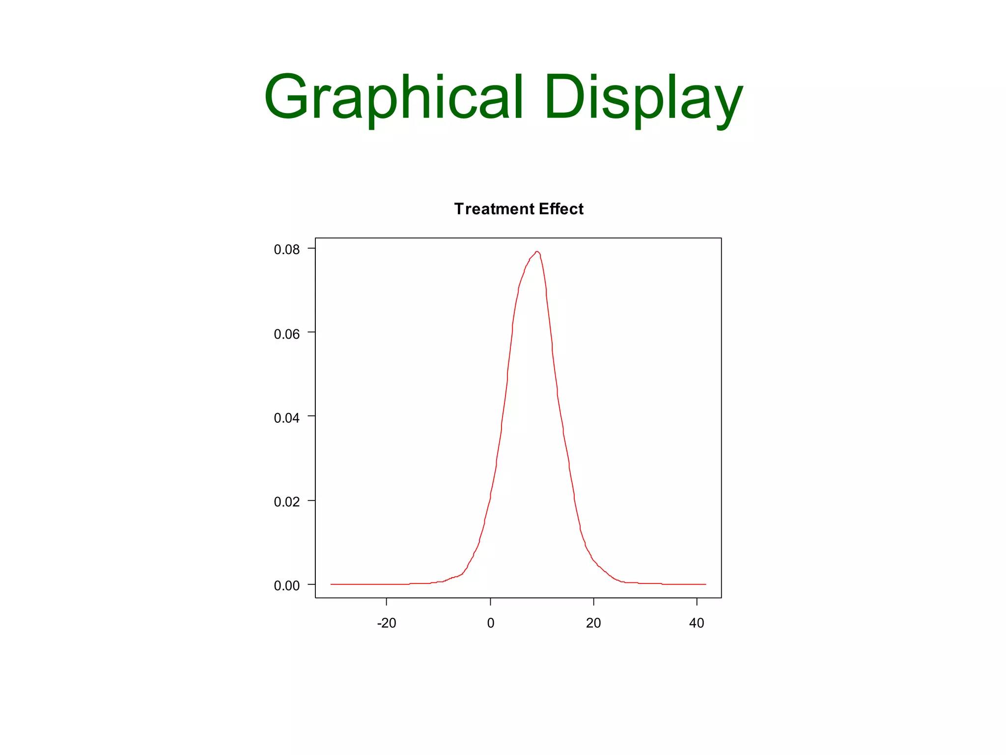
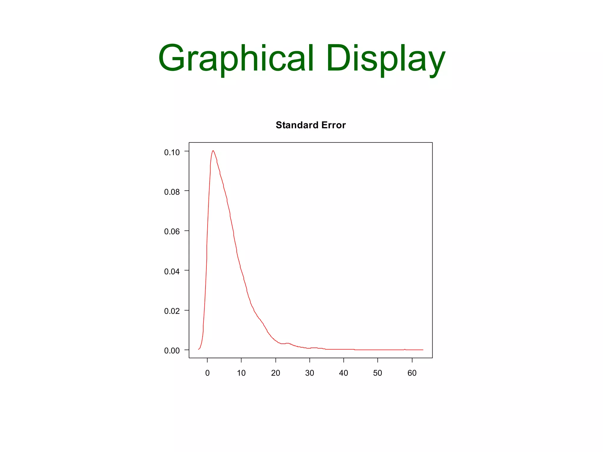
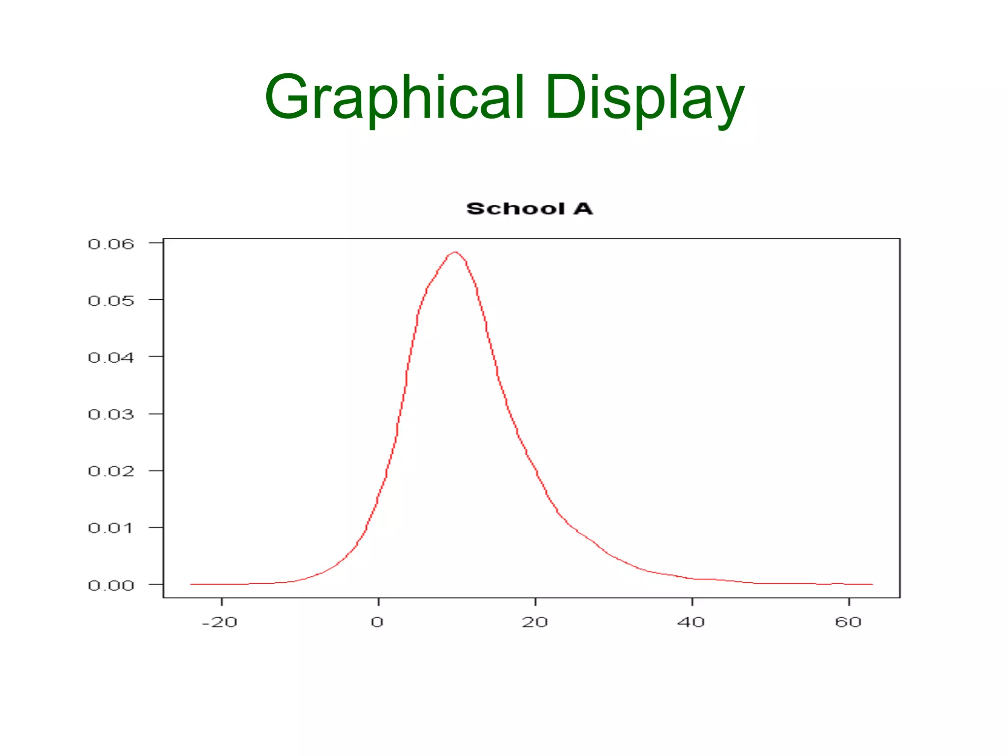
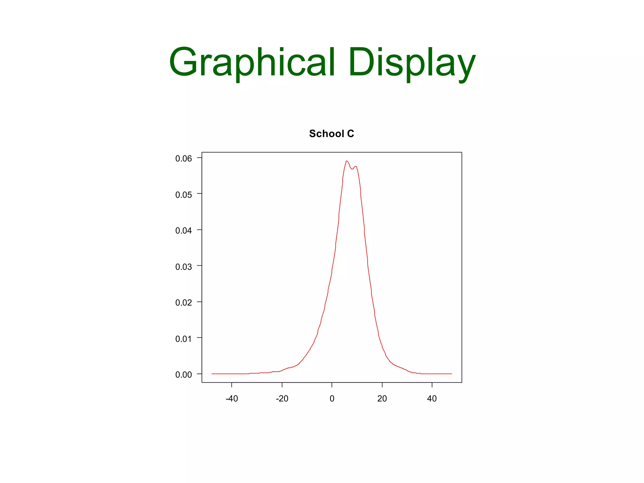
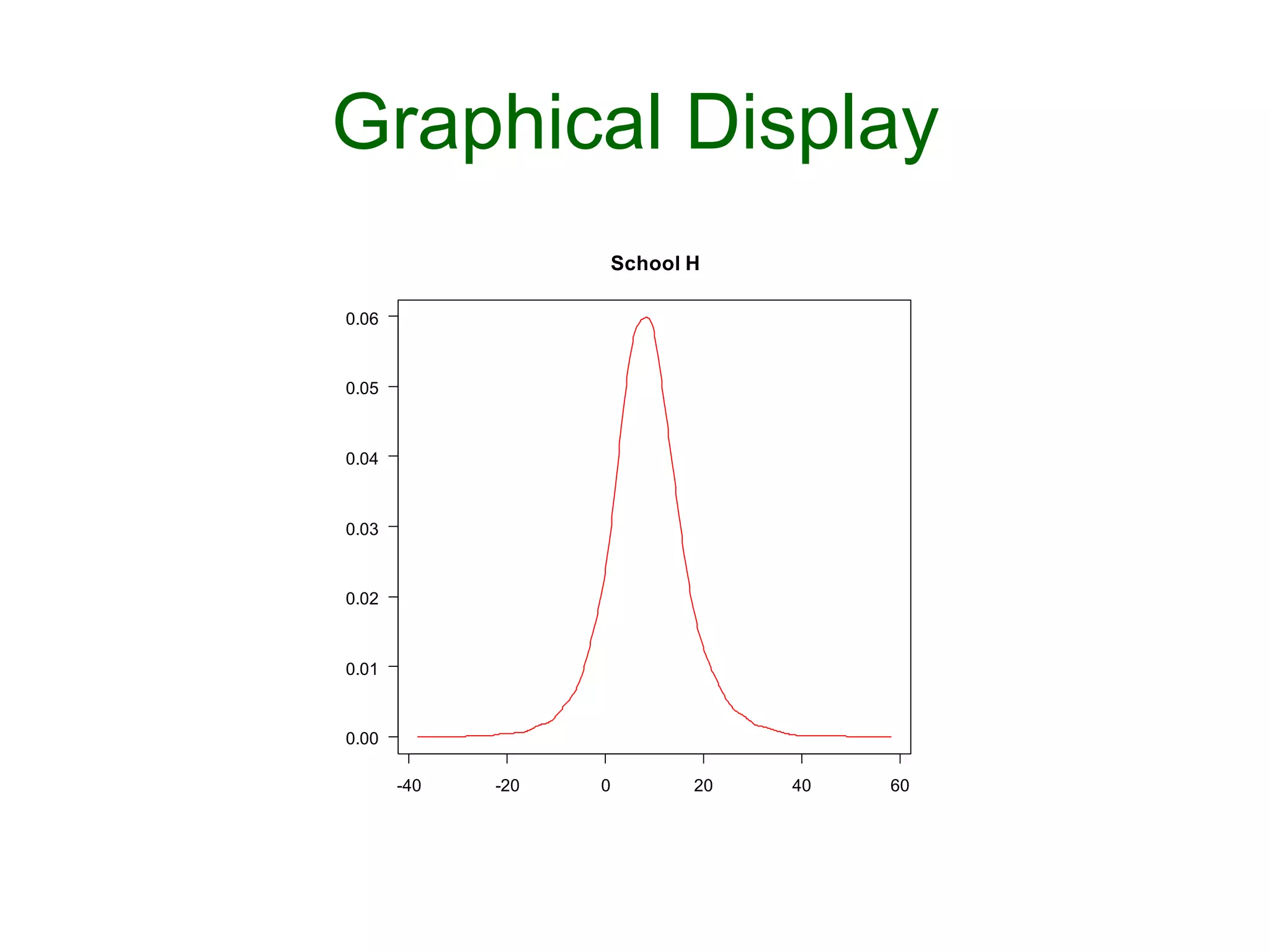
![Graphical Display
Ø plotDensity("mu.theta",las=1,
main = "Treatment Effect")
Ø plotDensity("sigma.theta",las=1,
main = "Standard Error")
Ø plotDensity("theta[1]",las=1,
main = "School A")
Ø plotDensity("theta[3]",las=1,
main = "School C")
Ø plotDensity("theta[8]",las=1,
main = "School H")](https://image.slidesharecdn.com/bayesianstatisticsintrousingr-130906103849-/75/Bayesian-statistics-intro-using-r-54-2048.jpg)


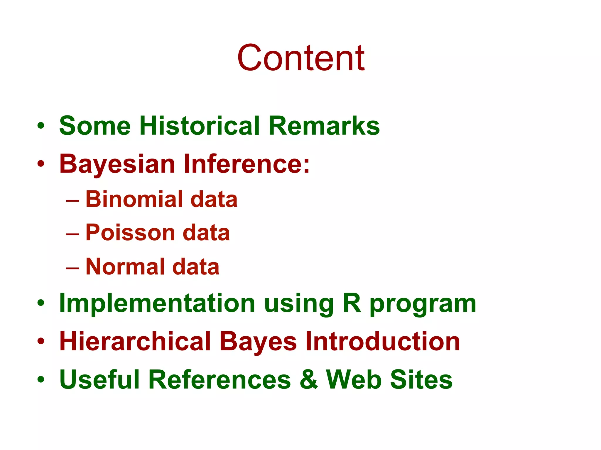
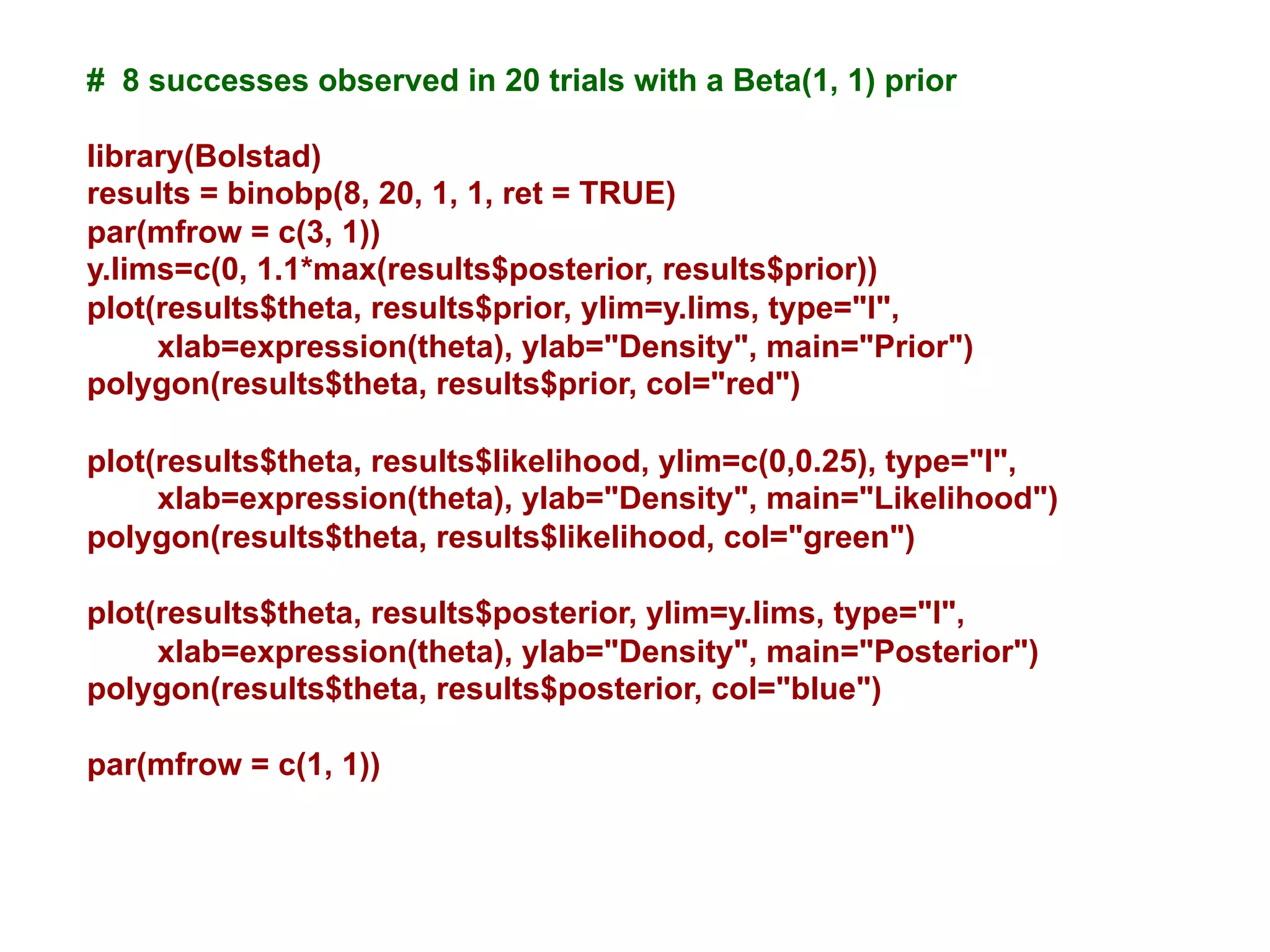
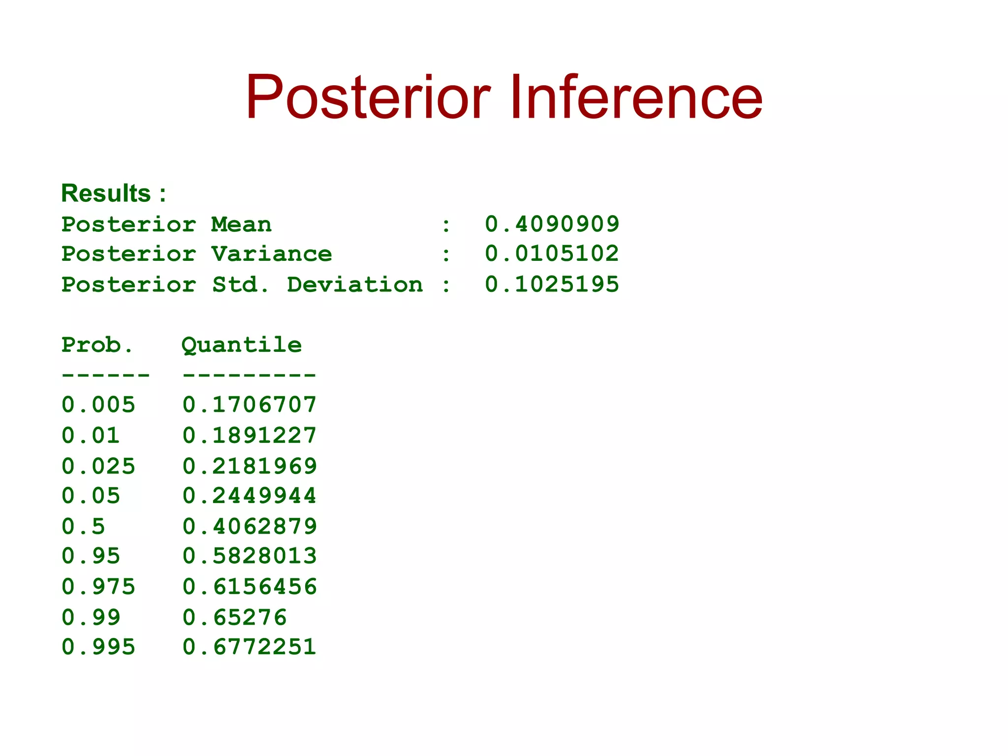
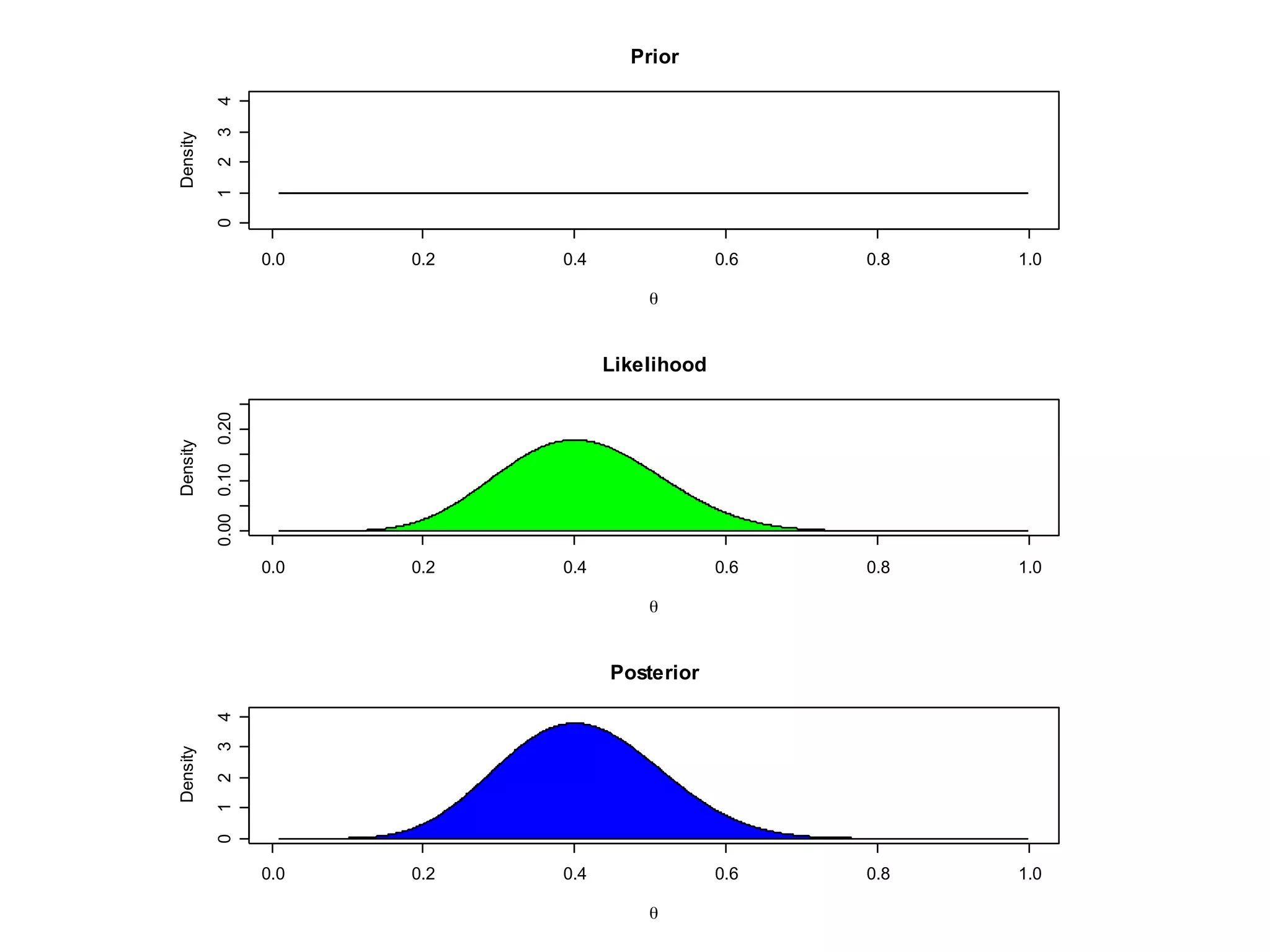
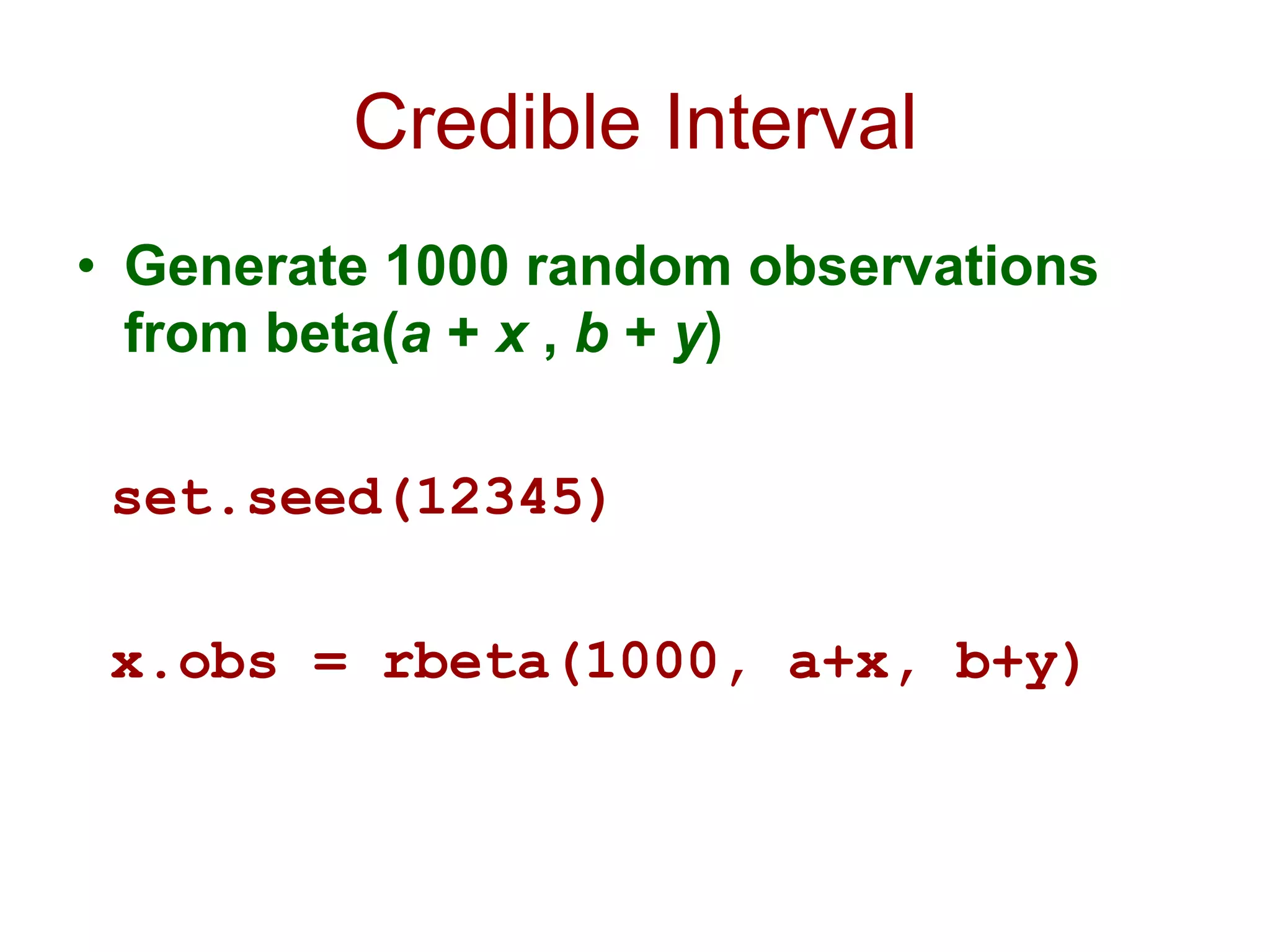
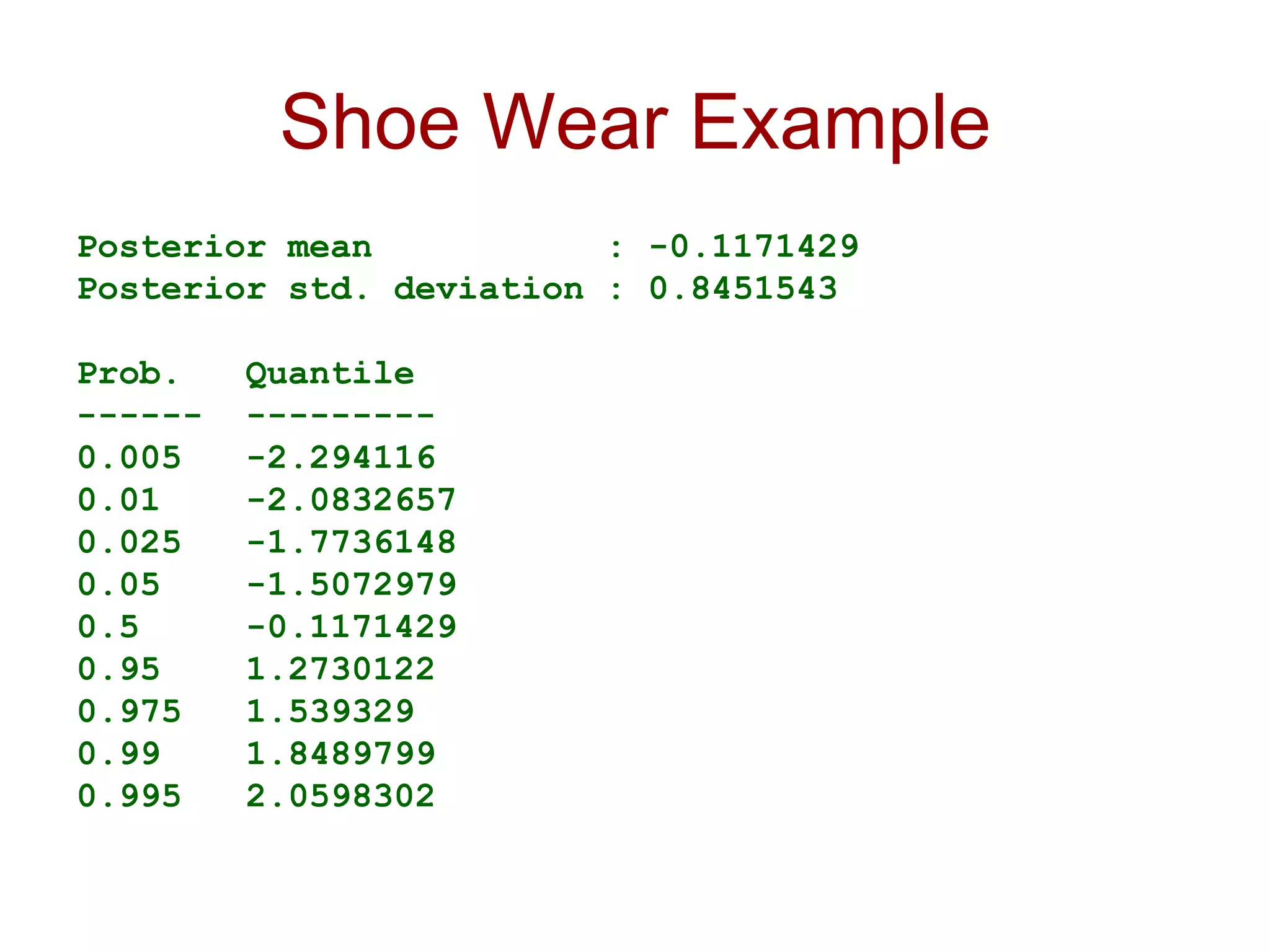
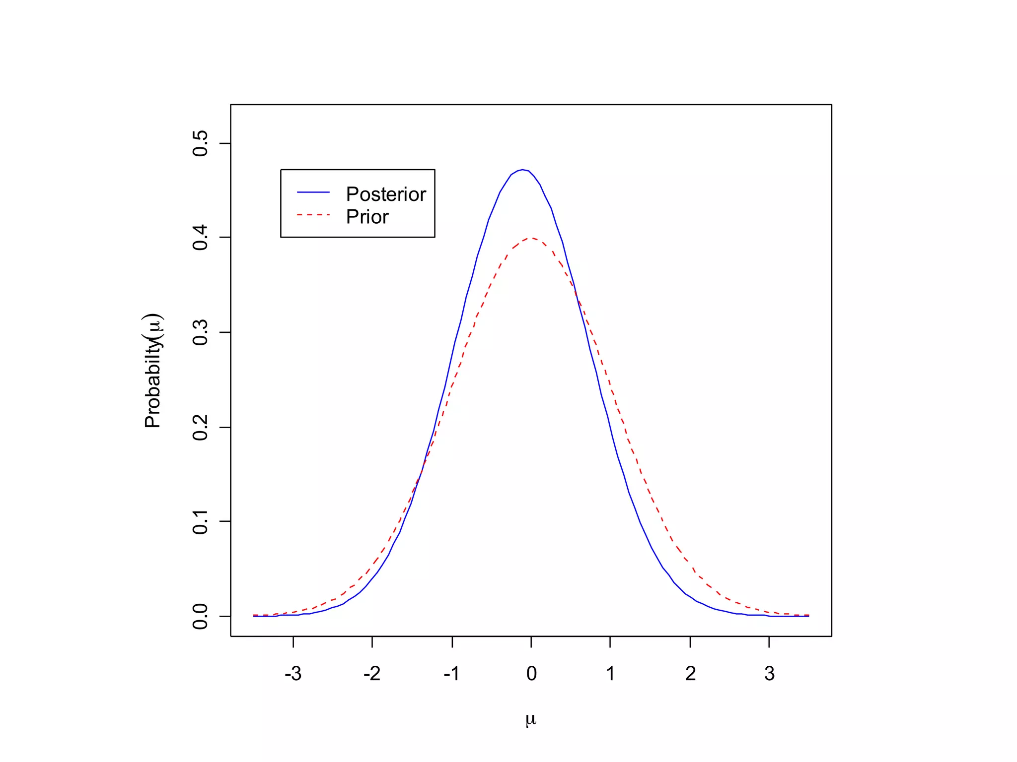
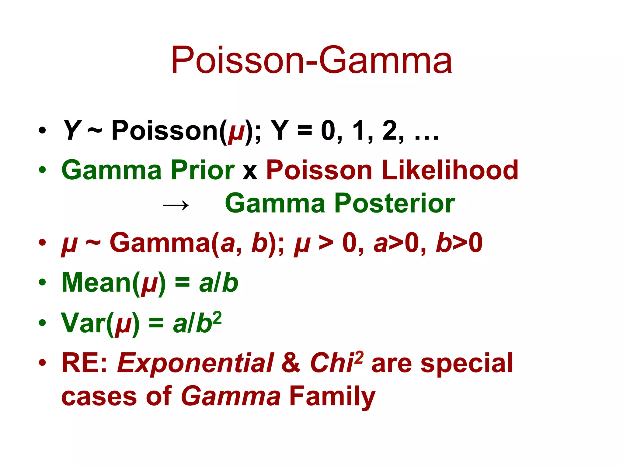
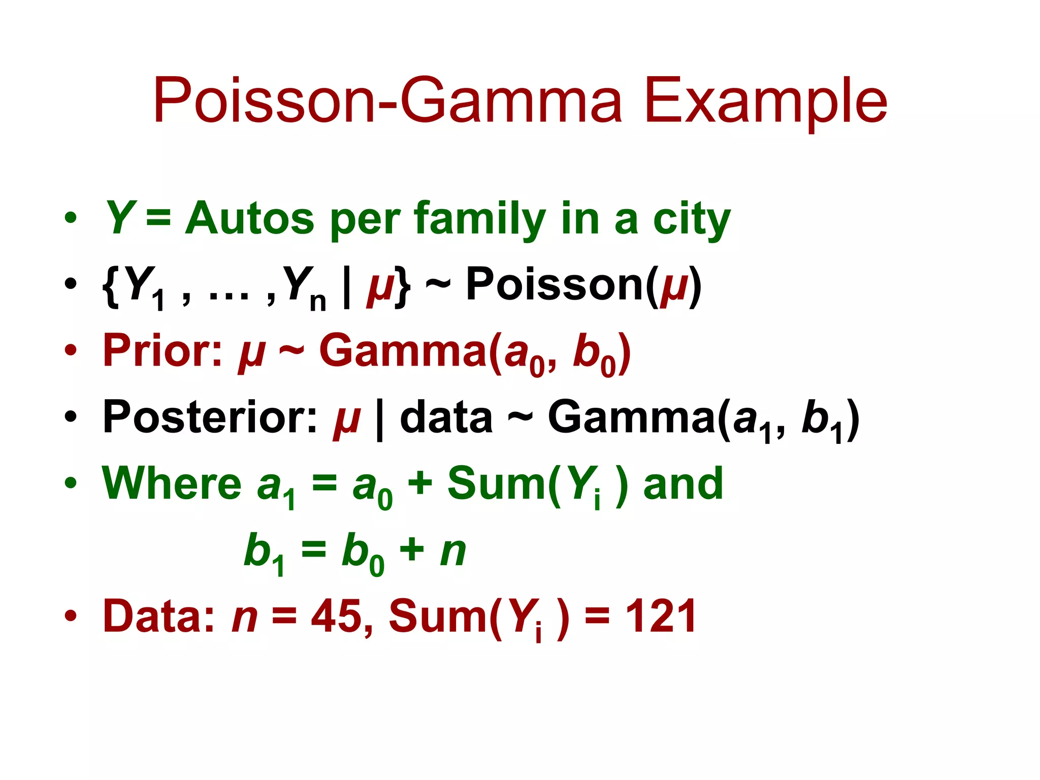
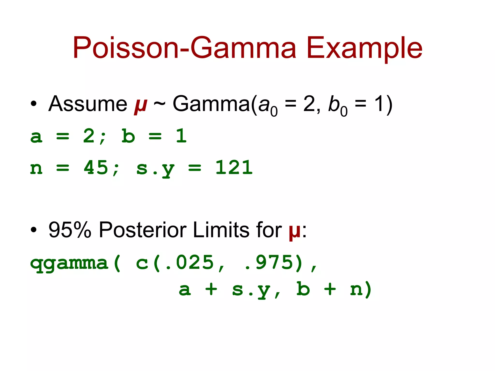
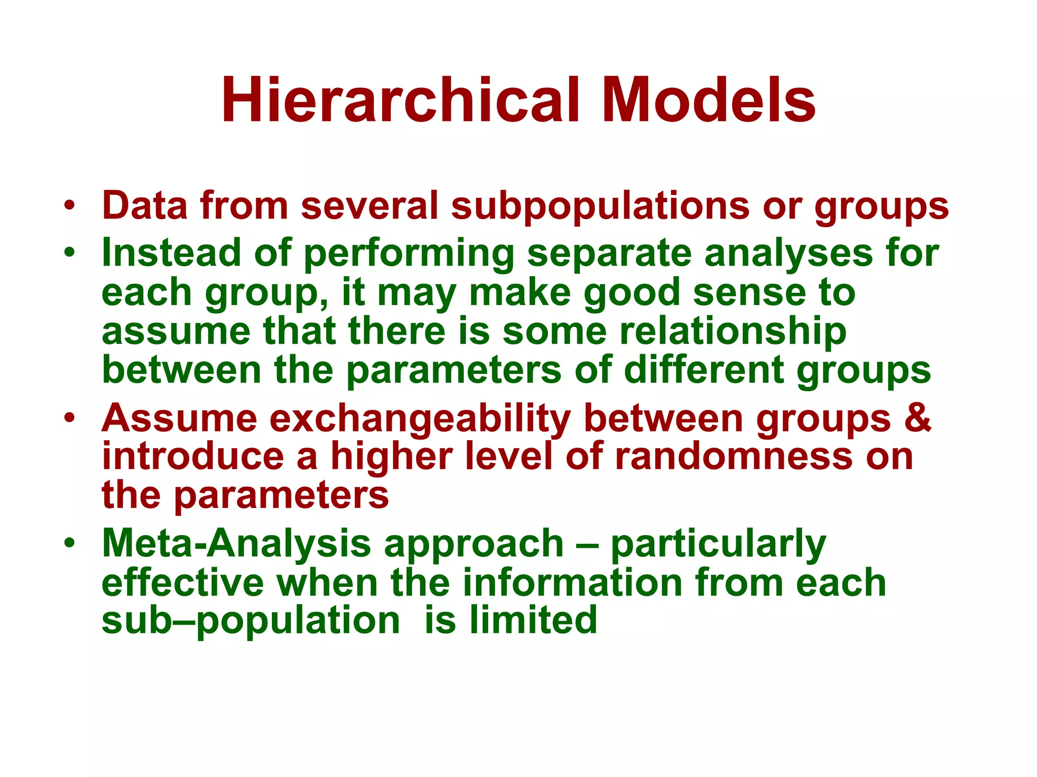
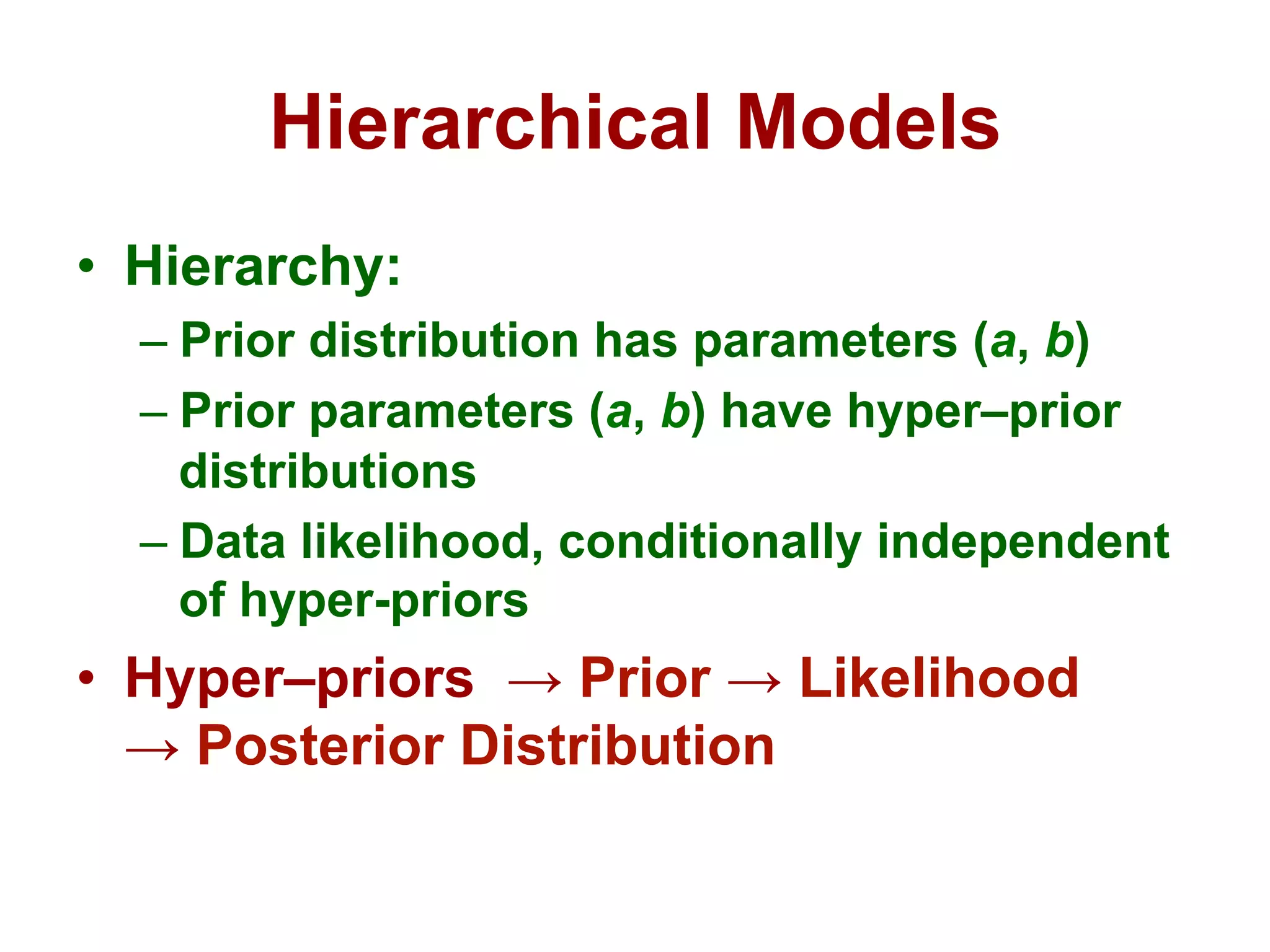
This document provides an introduction to Bayesian statistics using R. It discusses key Bayesian concepts like priors, likelihoods, posteriors, and hierarchical models. Specifically, it presents examples of Bayesian inference for binomial, Poisson, and normal data using conjugate priors. It also introduces hierarchical modeling through the eight schools example, where estimates of treatment effects across multiple schools are modeled jointly.