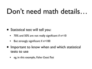
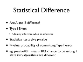
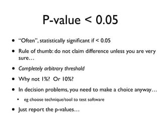
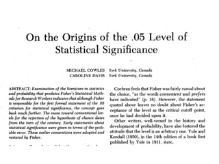
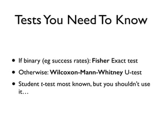
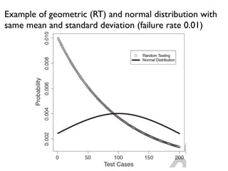
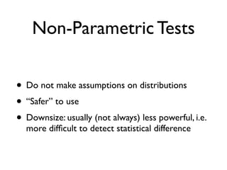
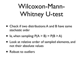
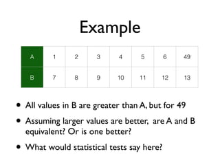
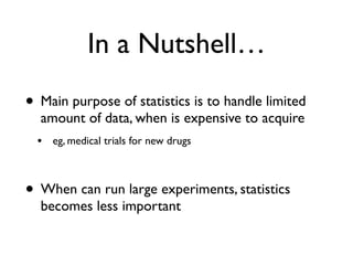
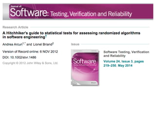
This document provides an introduction to statistics, data analysis, and visualization in R and Latex. It discusses why statistics are important for experiments and compares different statistical tests that can be used to analyze data, including the Fisher Exact test, Wilcoxon-Mann-Whitney U-test, and Student's t-test. It also addresses issues around sample sizes and distributions, emphasizing that statistics are useful for handling limited data and determining practical versus statistical significance.

1. Intro to Statistics, Data
Analysis andVisualisation
in R and Latex
Dr.Andrea Arcuri
Software Engineer Consultant, Scienta, Norway
Research Fellow, University of Luxembourg
aa@scienta.no

2. In This Seminar
• Why using statistics?
• Basic statistics
• eg, Wilcoxon-Mann-Whitney U-test
• Examples in R
• Automate table generation in Latex
• ie, avoid filling data by hand
• add statistics with just couple of lines of code…

3. Just an informal intro for
beginners…
quite complex topic if you
look at the details…

4. Focus on comparisons of testing techniques, tools and
algorithms
For empirical studies with human subjects, things are
bit different… (eg, constraints on sample size)

5. Why bother with
statistics?

6. Experiments
• Evaluate if new technique A is better than B
• eg, compared to the state-of-the-art
• code coverage, fault detection, etc
• Large experiments can be too time consuming
• Not just software testing
• most branches of engineering and science (medicine, biology,
etc.)

7. Statistics: have I run
enough experiments?

8. Randomised Algorithms
• Run twice, can get different results
• Many different kinds
• Random Testing (RT)
• Search-Based Software Testing (SBST)
• Some kinds of Dynamic Symbolic Execution (DSE)
• etc
• How many N runs with different seeds?

9. Case Study Selection
• Space Z of possible problem instances
• On some instances, technique A works fine (eg
better than B), but not on others
• How many N instances from Z to use?
• How can you select?
• even if unbias, maybe you just got lucky…
• Still probability involved

10. Motivating Example
• Two algorithms, A and B
• Run n=10 times, or 1 on n=10 different instances
• Binary output: pass or fail
• A: successful 7 times
• B: successful 5 times
• 20% of success rate difference
• Is A better than B???

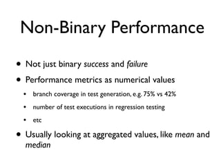
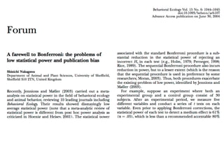
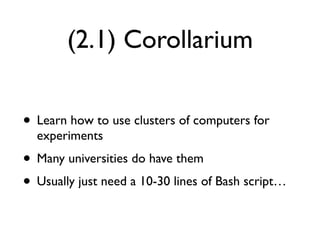
11. Probability
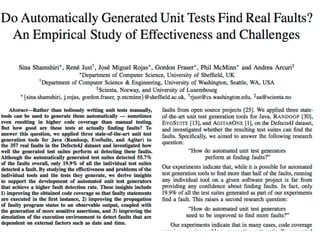
• Probability p in [0,1] of:
• a successful run in a randomised algorithm
• sampling/choosing an instance for which algorithm is successful
• k successes out of n runs/instances
• n-k failures
• order of k and n-k does not matter
• estimated success rate of p: r=k/n
• for n to infinite, r would converge to p

12. Binomial Distribution B(n,r)
• What is the probability P of having k successes
when I have n instance/runs with success rate r?
• P(B(n,r)=k) = bin(n,k) * rk * (1-r)(n-k)
any
order
n-k
failures
k
successes

13. Examples
• In R,“dbinom(k,n,r)”
• P(B(10,0.7)=7) = 0.26
• If real success rate is 70%, then there is only a 26% probability
of obtaining 7 successes out of 10 runs/instances
• But what if actual success rate was 50%?
• P(B(10,0.5)=7) = 0.11
• 26% > 11%, but still 11% not so unlikely…

14. The most likely
estimate r=k/n might
not have high
probability of being
correct

15. Comparing A with B
• A: P(B(10,0.7)=7) = 0.26
• B: P(B(10,0.5)=5) = 0.24
• P(B(10,.7)=7) * P(B(10,.5)=5) = 0.06
• only 6% probability that, if X has success rate 70% andY has
50%, then X obtains 7 successes andY 5

16. But what if…
• … A and B have exactly same success rate 60%?
• ie, got bit lucky with A, and bit unlucky with B
• P(B(10,.6)=7) * P(B(10,.6)=5) = 0.04
• 4% not so huge difference from 6%…
• What if B is actually better?
• less likely, but still possible

17. n=10
A: k=7
B: k=5
n=100
A: k=70
B: k=50
Probability (Z axis) of getting 70% successes with A and 50% for B
for different success rates of A and B (X and Y axes)
>0% that B is better
extremely unlikely that B was better

18. Don’t need math details…
• Statistical test will tell you:
• 70% and 50% are not really significant if n=10
• But strongly significant if n=100
• Important to know when and which statistical
tests to use
• eg, in this example, Fisher ExactTest

19. compareAB_n10 <- function(){
n = 10
ka = 7
kb = 5
m = matrix(c(ka,n-ka,kb,n-kb),2,2)
fisher.test(m)
}
compareAB_n100 <- function(){
n = 100
ka = 70
kb = 50
m = matrix(c(ka,n-ka,kb,n-kb),2,2)
fisher.test(m)
}

20. p-value can give you an hint on
whether you can say the two
compared A and B are different
eg, < 0.05

21. What Statistical Tools
to Use?
• Many options, open-source and commercial
• Two most used/popular: R and Python
• R: open source, specific for statistics, large
community
• Python: open source, general scripting language,
good libraries for statistics

22. How to Choose?
• If you already know Python outside of statistics,
go for Python
• If not, R might be safest option (de-facto standard)
• Both language have their quirks
• Personally I use R, but it does not mean R is a
good language…
• Most important feature: need to have scripting,
not just a GUI

24. Programming with a dynamically typed language (eg, R
and Python) can be a painful experience…
… but scripts for statistics are usually short and not
complex…
… and re-used paper after paper…

25. Statistical Tests

26. Statistical Difference
• Are A and B different?
• Type I Error:
• Claiming difference when no difference
• Statistical tests give p-value
• P-value: probability of committing Type I error
• eg, p-value=0.1 means 10% chance to be wrong if
state two algorithms are different

27. P-value < 0.05
• “Often”, statistically significant if < 0.05
• Rule of thumb: do not claim difference unless you are very
sure…
• Completely arbitrary threshold
• Why not 1%? Or 10%?
• In decision problems, you need to make a choice anyway…
• eg choose technique/tool to test software
• Just report the p-values…

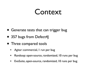
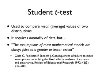
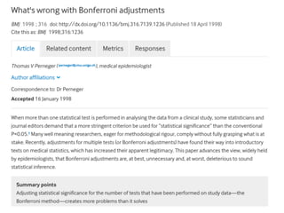
29. More than 100 years old
• Student [W. S. Gosset]. The probable error of a
mean. Biometrika, 1908
• about t-test:“three times the probable error in the normal curve,
for most purposes, would be considered significant”
• Fisher, R.A. Statistical methods for research workers.
Edinburgh: Oliver & Boyd, 1925.
• just rounding 0.0456 to 0.05
• “rejection level of 3PE is equivalent to two times the SD (in modern
terminology, a z score of 2)”

30. TestsYou Need To Know
• If binary (eg success rates): Fisher Exact test
• Otherwise: Wilcoxon-Mann-Whitney U-test
• Student t-test most known, but you shouldn’t use
it…

31. Fisher Exact Test
• In R: fisher.test(m)
• m is a 2x2 matrix
• Check if can claim
different success rates
# Success for A # Failures for A
# Success forB # Failures for B

32. Example
• Automated Bug Fixing
• You somehow sample N bugs to repair, with as little
bias as possible
• Want to know if your novel technique A is better
than state of the art B
• Run experiments with N=30
• A repairs 20, whereas B repairs 15
• Can claim with high confidence that A is better?

33. compareAB_bugFixing <- function(){
n = 30
ka = 20
kb = 15
m = matrix(c(ka,n-ka,kb,n-kb),2,2)
fisher.test(m)
}

34. But does it matter that
not enough evidence to
claim A is better?

35. Not really…
• Evidence of 5 bugs fixed by A but not B
• Can’t say A is better, but can say A is useful
• Techniques can be combined/integrated
• Given a domain (eg bug fixing), no single paper
can solve all instances

36. “Similar” Example
• Still Automated Bug Fixing
• Now A and B are randomised (eg Genetic
Programming)
• Single bug, run experiments 30 times
• A repairs 20 times, whereas B repairs 15 times
• Can claim with high confidence that A is better?
• Can claim that A is useful?

37. Bit different now…
• A better? No (recall high p-value 0.29)
• A useful? Arguably no, i.e. equivalent to B
• In this case, warranted to run some more
experiments before trying to publish it…

38. But what if…
• … I am comparing randomised algorithms on
many problem instances?
• Typical case of SBST and when comparing with RT

40. Context
• Generate tests that can trigger bug
• 357 bugs from Defect4J
• Three compared tools
• Agitar: commercial, 1 run per bug
• Randoop: open-source, randomized, 10 runs per bug
• EvoSuite, open-source, randomized, 10 runs per bug

41. Results
• Bugs found only by…
• Agitar: 28
• Random: 12
• EvoSuite: 35
• No technique subsumes the others
• In many cases, Randoop/EvoSuite found bug only
in a subset of the 10 runs…

42. So 2 Steps Analysis
• On single instances to check A vs B performance
• need to take into account randomness
• On whole case study
• based on how was selected, from random sample can infer/
estimate performance on whole domain
• more on this later…

43. Non-Binary Performance
• Not just binary success and failure
• Performance metrics as numerical values
• branch coverage in test generation, e.g. 75% vs 42%
• number of test executions in regression testing
• etc
• Usually looking at aggregated values, like mean and
median

44. Student t-test
• Used to compare mean (average) values of two
distributions
• It requires normality of data, but…
• “The assumptions of most mathematical models are
always false to a greater or lesser extent”
• Glass G, Peckham P, Sanders J. Consequences of failure to meet
assumptions underlying the fixed effects analyses of variance
and covariance. Review of Educational Research 1972; 42(3):
237–288.

45. Normal Distribution
Fully defined by two
properties: mean
and standard
deviation
Many phenomena in
nature fit in a normal
distribution

46. Example
• Generating n test cases before finding bugs
• Randomised algorithm, so n can be represented as
random variable
• Can n be normally distributed?
• NEVER: n<0 is impossible, and discrete value (ie,
no fraction of tests, e.g. 1.3)

47. t-test (continued.)
• The Central Limit Theorem (CLT) states that the
sum of n random variables converges to a normal
distribution as n increases
• t-test internally uses sums of random variables
• Often, already with n=30 the t-test is robust to
deviation from normality

48. CLT Example
• Rolling a dice
• What is probability
distribution of a 6 face
dice?
• Each value has 16%
probability
• Definitively not normal

49. CLT (continued.)
• But what is the
probability of the
sum of n dices?
• Even with as low as
n=2, it starts to look
normal…

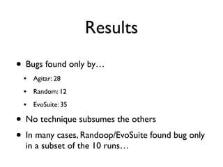
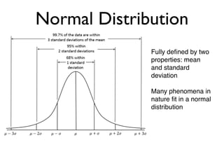
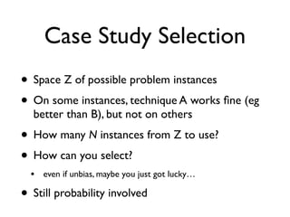
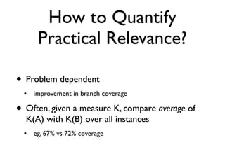
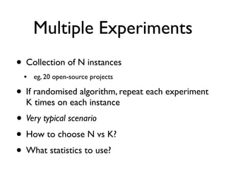
50. A More Relevant Example
• Unit test generation (EvoSuite) for code coverage
• Sample 100 projects at random from SourceForge
(the SF100 corpus)
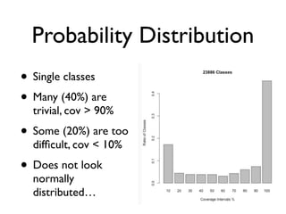
• Coverage [0%,100%] for single classes
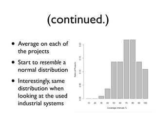
• Average/mean coverage on the 100 projects
• recall sum of n variables divided/scaled by n

52. Probability Distribution
• Single classes
• Many (40%) are
trivial, cov > 90%
• Some (20%) are too
difficult, cov < 10%
• Does not look
normally
distributed…

53. (continued.)
• Average on each of
the projects
• Start to resemble a
normal distribution
• Interestingly, same
distribution when
looking at the used
industrial systems

54. What about checking
normality?
• Check normality before using t-test
• Shapiro-Wilk test
• hypothesis normality, p-value to check if can reject it
• Few problems with this approach:
• increase error, as doing 2 tests now
• small n: everything looks normal
• some algorithms have known non-normal distributions

55. Random Testing
• Often used as a baseline when evaluating new
techniques
• Easy to implement, in some cases can give good
results
• Eg, sample n test cases until trigger a bug
• n follows a geometric distribution, not a normal one

56. Example of geometric (RT) and normal distribution with
same mean and standard deviation (failure rate 0.01)

57. Non-Parametric Tests
• Do not make assumptions on distributions
• “Safer” to use
• Downsize: usually (not always) less powerful, i.e.
more difficult to detect statistical difference

58. Wilcoxon-Mann-
Whitney U-test
• Check if two distributions A and B have same
stochastic order
• Ie, when sampling: P(A > B) = P(B > A)
• Look at relative order of sampled elements, and
not their absolute values
• Robust to outliers

59. Example
• All values in B are greater than A, but for 49
• Assuming larger values are better, are A and B
equivalent? Or is one better?
• What would statistical tests say here?
A 1 2 3 4 5 6 49
B 7 8 9 10 11 12 13

60. comparisonTandU <- function(){
a = c(1,2,3,4,5,6,49)
b = c(7,8,9,10,11,12,13)
cat("Mean a: ", mean(a), "n")
cat("Mean b: ", mean(b), "n")
print(wilcox.test(a,b))
print(t.test(a,b))
}
Some mean 10,
so no difference
for t-test
Strong difference
for U-test

61. Which One To Use?
• If few data (ie low n):
• t-test might not be robust to deviation from normality
• U-test might be not enough powerful
• If lot of data
• t-test fine even if data is not normal (Central Limit Theorem)
• U-test becomes enough powerful

62. (continued.)
• If not enough data
• need to study details of statistics, and choose the right test
• eg, empirical study with 20-30ish students
• If lot of data
• does not matter so much what you use (eg t-test vs. U-test)
• eg, test data generation on cluster of computers

63. So If In Doubts…
• … just try to increase the amount of data!
• run experiments for longer
• use cluster of computers
• Not always possible:
• human subjects
• industrial case studies

64. In a Nutshell…
• Main purpose of statistics is to handle limited
amount of data, when is expensive to acquire
• eg, medical trials for new drugs
• When can run large experiments, statistics
becomes less important

65. Side-effects
With a lot of data…
… every difference, even if tiny, becomes statistically
significant
eg, very easy to get p-value < 0.05

66. Wrong Approach
• Run experiments
• Compare A with B
• Use statistics
• p-value < 0.05 (or any other threshold)
• Claim contribution because results are statistically
significant

67. A Better Approach
• Run experiments on A and B
• Is the difference of practical significance?
• this is problem dependent, e.g. enough branch coverage
improvement
• If yes: do statistical tests to check if you had
enough data
• If not: who cares of p-values…

68. How to Quantify
Practical Relevance?
• Problem dependent
• improvement in branch coverage
• Often, given a measure K, compare average of
K(A) with K(B) over all instances
• eg, 67% vs 72% coverage

69. Issues With Averages
• diff = mean(K(A)) - mean(K(B))
• Would ignore variability in the data
• eg if high standard deviation
• Improvement from 1% to 3% is not the same as
from 91% to 93%, although still diff=2%
• Issue if different order of measures, e.g.
• easy problems: e.g.A=10 vs B=20 test cases
• difficult problems: e.g.A=200,000 vs B=100,000
• Skewed results if outliers

70. Standardised Effect Sizes
• Independent from unit of measure
• robust if high variability in the instances of the case study
• Single measure, which takes into account also
variability
• Easier to compare among studies

71. Main Effect Sizes
• Odds Ratio
• for dichotomous results (eg success/failure)
• Cohen d
• most known, but “makes sense” only if data is normal, so quite
seldom… plus, difficult to interpret
• Vargha and Delaney A12 measure
• non-parametric, very easy to interpret
• personally, the one I use 99% of the times…

72. Odds Ratio
“measure of how many times greater the odds are
that a member of a certain population will fall into
a certain category than the odds are that a
member of another population will fall into that
category”

73. (continued)
• If same success rate, odds ratio = 1
• Automatically computed with Fisher test

74. Cohen d
• Difference in mean divided by pooled standard
deviation
• Larger mean difference: greater d
• Smaller standard deviation: greater d
• If no difference, d=0

75. (continued.)
standard deviation
(SD) has special
characteristics in
normal distribution
but in other
distributions, dividing
by SD can be
meaningless

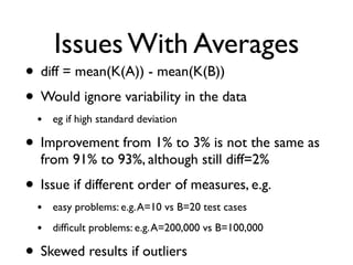
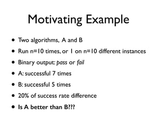
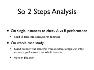
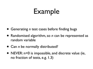
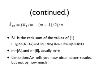
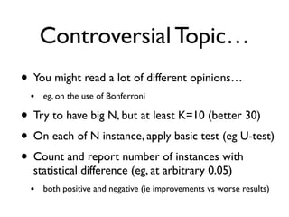
77. Vargha-Delaney A Measure
• Non-parametric
• A12 defines probability [0,1] that running
algorithm (1) yields higher values than running
another algorithm (2).
• If the two algorithms are equivalent, then A12=0.5
• Eg,A12=0.7 means 70% probability that (1) gives
better results

78. (continued.)
• R1 is the rank sum of the values of (1)
• eg,A={42,11,7} and B={1,20,5}, then R1=sum(6,4,3)=13
• m=|A|, and n=|B|, usually m=n
• Limitation:A12 tells you how often better results,
but not by how much

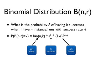
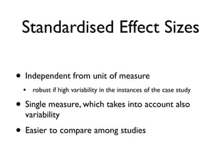
79. R Code For A12 Measure
measureA <- function(a,b){
r = rank(c(a,b))
r1 = sum(r[seq_along(a)])
m = length(a)
n = length(b)
A = (r1/m - (m+1)/2)/n
return(A)
}

80. On t-test vs. U-test
• Both are fine for statistical tests
• Can interpret U-test with A12
• If data not normal, t-test is still fine (Central Limit
Theorem), but NOT the Cohen d
• Having A12 is a good reason to choose U-test over
t-test
• Still can use both (they measure different things)

81. For Large Experiments…
• p-values get smaller and smaller
• NOT the standardised effect sizes
• they just get more precise
• you ll not see much difference between n=100 and n=1,000,000

82. The Wrath of Bonferroni
• When running several tests, increase Type I error
• ie high probability of wrongly rejecting at least one null
hypothesis
• Bonferroni adjustment: reduce threshold for
statistical significance based on number k of tests
• eg 0.05/k
• I NEVER use it (long story)… but, if reviewers ask
for it…

85. Multiple Experiments
• Collection of N instances
• eg, 20 open-source projects
• If randomised algorithm, repeat each experiment
K times on each instance
• Very typical scenario
• How to choose N vs K?
• What statistics to use?

86. Controversial Topic…
• You might read a lot of different opinions…
• eg, on the use of Bonferroni
• Try to have big N, but at least K=10 (better 30)
• On each of N instance, apply basic test (eg U-test)
• Count and report number of instances with
statistical difference (eg, at arbitrary 0.05)
• both positive and negative (ie improvements vs worse results)

87. More Positive or Negative
Cases?
• Calculate effect size A12 on each of the N instances
• Report average/median effect sizes
• Statistics on whether the N values of A12 are
symmetric around 0.5
• wilcox.test(c(a1,a2,a3,…,an), mu=0.5)

88. How ToVisualise The
Data and Results of the
Statistical Tests?

89. Java Enterprise Edition Support in Search-Based JUnit Test Generation, Arcuri and Fraser, SSBSE’16

90. Tables
• Good way to show statistical tests
• a row for each problem instance (if not too many)
• a column for effect size (in bold if p-value < 0.05)
• a column for p-value
• a final row with average values
• Of course, many more options (eg, graphs,
boxplots, etc.)

91. RaiseYour Hand If…
• you have ever filled a table by hand, e.g. in Microsoft
Word, and …
• data is invalid, get new data, refill table by hand…
• … again and again…
• (extra points if at 4am of a conference deadline night)

92. DO NOT DO IT
• Unless it is trivial small (eg 2x2 table)
• Very error prone (especially at 4am)
• If you see colleague/student doing it, hit them
• or use any other form of legal punishment in your country
• they will be grateful, one day…
• Invest time in learning Latex and R
• or any other equivalent combination

93. From Scripts to PDF
• Given some data X on file (eg CSV)
• Use scripts (R/Python) to load it
• Create “textual” representation of table, and save
it to a file K
• Automatically import K in your paper document
(eg if written in Latex)
• Generate PDF from your paper document

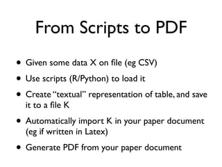
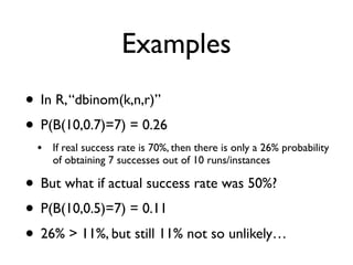
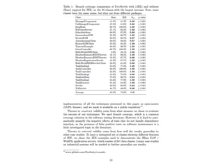
94. begin{table}[t!]
centering
caption{label{table:selection}
Branch coverage comparison of evo with (JEE) and without (Base)
support for JEE, on the 25 classes with the largest increase.
Note, some classes have the same name, but they are from different
packages.
}
scalebox{0.85}{
input{generated_files/tableSelection.tex}
}
end{table}
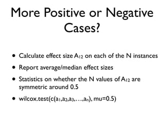
To get a better picture of the importance of handling JEE features,
Table~ref{table:selection} shows detailed data on the 25 challenging
classes where JEE handling had most effect: On these classes, the
paper.tex

95. begin{tabular}{ l @{hspace{0.5cm}}r@{hspace{0.5cm}}r@{hspace{0.5cm}} r@{hspace{0.5cm}}r }
toprule
Class & Base & JEE & $hat{A}_{12}$ & $p$-value
midrule
ManagedComponent & 14.3% & 41.2% & {bf 0.96} & {bf $le 0.001$}
UnManagedComponent & 47.0% & 51.6% & {bf 0.80} & {bf $le 0.001$}
ItemBean & 89.7% & 100.0% & {bf 1.00} & {bf $le 0.001$}
HATimerService & 57.1% & 93.3% & {bf 1.00} & {bf $le 0.001$}
SchedulerBean & 60.0% & 97.3% & {bf 0.98} & {bf $le 0.001$}
IntermediateEJB & 33.3% & 66.7% & {bf 1.00} & {bf $le 0.001$}
SecuredEJB & 80.0% & 98.7% & {bf 0.97} & {bf $le 0.001$}
AsynchronousClient & 20.0% & 29.3% & {bf 0.97} & {bf $le 0.001$}
RemoteEJBClient & 25.0% & 58.3% & {bf 1.00} & {bf $le 0.001$}
TimeoutExample & 60.0% & 99.3% & {bf 1.00} & {bf $le 0.001$}
GreetController & 66.7% & 100.0% & {bf 1.00} & {bf $le 0.001$}
HelloWorldJMSClient & 4.9% & 23.1% & {bf 1.00} & {bf $le 0.001$}
MemberResourceRESTService & 19.1% & 69.2% & {bf 1.00} & {bf $le 0.001$}
MemberResourceRESTService & 19.3% & 67.7% & {bf 0.96} & {bf $le 0.001$}
MemberRegistrationServlet & 18.2% & 87.1% & {bf 1.00} & {bf $le 0.001$}
HelloWorldMDBServletClient & 26.0% & 61.3% & {bf 0.99} & {bf $le 0.001$}
TaskDaoImpl & 55.6% & 77.8% & {bf 1.00} & {bf $le 0.001$}
AuthController & 30.0% & 100.0% & {bf 1.00} & {bf $le 0.001$}
TaskController & 42.9% & 100.0% & {bf 1.00} & {bf $le 0.001$}
TaskDaoImpl & 55.6% & 75.0% & {bf 0.96} & {bf $le 0.001$}
TaskListBean & 75.0% & 96.7% & {bf 0.93} & {bf $le 0.001$}
TaskDaoImpl & 55.6% & 77.8% & {bf 1.00} & {bf $le 0.001$}
TaskResource & 55.4% & 84.3% & {bf 1.00} & {bf $le 0.001$}
Servlet & 40.0% & 60.9% & {bf 0.92} & {bf $le 0.001$}
XAService & 44.7% & 49.3% & {bf 0.96} & {bf $le 0.001$}
midrule
Average & 43.8% & 74.6% & 0.98 &
bottomrule
end{tabular}

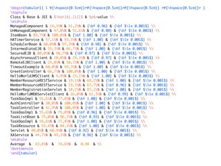
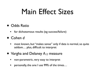
96. bestSelectionTable <- function(){
dt <- read.table(gzfile(SELECTION_ZIP_FILE),header=T)
TABLE = paste(GENERATED_FILES,"/tableSelection.tex",sep="")
unlink(TABLE)
sink(TABLE, append=TRUE, split=TRUE)
cat("begin{tabular}{ l @{hspace{0.5cm}}r@{hspace{0.5cm}}r@{hspace{0.5cm}} r@{hspace{0.5cm}}r }toprule","n")
cat("Class & Base & JEE & $hat{A}_{12}$ & $p$-value ","n")
cat("midrule","n")
Bv = c(); Fv = c(); Av = c()
selection = getBestClassesSelection(dt,25)
projects = sort(unique(dt$group_id))
for(proj in projects){
classes = unique(dt$TARGET_CLASS[dt$group_id==proj])
classes = sort(classes[areInTheSubset(classes,selection)])
for(cl in classes){
mask = dt$group_id==proj & dt$TARGET_CLASS==cl
base = dt$BranchCoverage[mask & dt$configuration_id=="Base"]
pafm = dt$BranchCoverage[mask & dt$configuration_id=="JEE"]
a12 = measureA(pafm,base)
w = wilcox.test(base,pafm,exact=FALSE,paired=FALSE)
pv = w$p.value
if(is.nan(pv)) {pv = 1}
stat = pv < 0.05
if(pv < 0.001){ pv = "le 0.001"
} else { pv = formatC(pv,digits=3,format="f")}
cat(getClassName(cl))
cat(" & “); cat(formatC(100*mean(base),digits=1,format="f"),"%",sep="")
cat(" & “); cat(formatC(100*mean(pafm),digits=1,format="f"),"%",sep="")
a12Formatted = formatC(a12,digits=2,format="f")
cat(" & ")
if(!stat) {
cat(a12Formatted, " & ")
cat("$",pv,"$",sep="")
} else {
cat("{bf ",a12Formatted,"} & ",sep="")
cat("{bf $",pv,"$}",sep="")
}
cat(" n")
Bv = c(mean(base),Bv)
Fv = c(mean(pafm),Fv)
Av = c(a12,Av)
}
}
cat("midrule","n")
avgB = paste(formatC(100*mean(Bv),digits=1,format="f"),"%",sep="")
avgF = paste(formatC(100*mean(Fv),digits=1,format="f"),"%",sep="")
avgA = formatC(mean(Av),digits=2,format="f")
cat("Average & ", avgB," & ",avgF," & ",avgA," & n")
cat("bottomrule","n")
cat("end{tabular}","n")
sink()
}
analyze.R
actual statistics is
just couple of lines

97. When generating tables/
graphs in R/Latex, adding
statistics is trivial!
Data change? No problem:
$> bestSelectionTable()
$> pdflatex paper.tex

99. ROI of learning Latex/R
• Steep learning curve
• Will save you lot of time, year after year
• Most analyses in the papers are similar
• i.e. copy&paste R scripts from paper to paper
• If you are doing a PhD in Software Engineering,
writing 50-100 lines of R should not be a big
problem…

100. Conclusion
• Just a brief, high level introduction
• Many more things to cover
• Few take away lessons…

101. (1) Statistics Is Not
Mumbo Jumbo
• If used in all fields of science and engineering for
more than 100 years, there must be a reason…
• ISSTA’13 review:“…1217 is simply a statistically estimated (not
real) lower bound based on inspection of only 20 classes! The
authors should just report exactly what they confirmed on the
sampled 20 cases rather than using statistically estimated
numbers.”
• … not a big deal, you just submit to EMSE…

102. (2) The more data,
the better
• If in doubt…
• t-test or U-test?
• Is it wrong to skip Bonferroni?
• Do I really have to learn all that math stuff?
• Well, the more data, the less important the
statistical tests become
• If can’t have experiments with 1000 students (or
industrial systems), maybe can on 1000 open-
source projects

103. (2.1) Corollarium
• Learn how to use clusters of computers for
experiments
• Many universities do have them
• Usually just need a 10-30 lines of Bash script…

104. (3) Main Statistics To Use
• Fisher Exact test with odds ratio
• U-test with A12 effect sizes
• There are more, but those are good starting points
• Remember 0.05 threshold is arbitrary…

105. (4) Automation
• Automate the generation of tables/graphs
• Learn R/Python and Latex
• When generation is automated, adding statistics
takes just a couple of minutes