It is an experimental design problem in which there are two Poisson sources with two possible and known rates, and one counter. Through a switch, the counter can observe the sources individually or the counts can be combined so that the counter observes the sum of the two. The sensor scheduling problem is to determine an optimal proportion of the available time to be allocated toward individual and joint sensing, under a total time constraint. Two different metrics are used for optimization: mutual information between the sources and the observed counts, and probability of detection for the associated source detection problem. Our results, which are primarily computational, indicate similar but not identical results under the two cost functions.

1. Sensing Method for Two-Target
Detection in Time-Constrained Vector
Poisson Channel
Muhammad Fahad, Member, IEEE
Department of Applied Computing
Michigan Technological University
Houghton, MI 49931, USA
mfahad@mtu.edu
Daniel R. Fuhrmann, Fellow, IEEE
Department of Applied Computing
Michigan Technological University
Houghton, MI 49931, USA
fuhrmann@mtu.edu
Abstract
It is an experimental design problem in which there are two Poisson sources with two
possible and known rates, and one counter. Through a switch, the counter can observe
the sources individually or the counts can be combined so that the counter observes the
sum of the two. The sensor scheduling problem is to determine an optimal proportion of
the available time to be allocated toward individual and joint sensing, under a total time
constraint. Two different metrics are used for optimization: mutual information between
the sources and the observed counts, and probability of detection for the associated
source detection problem. Our results, which are primarily computational, indicate
similar but not identical results under the two cost functions.
Index Terms
sensor scheduling, vector Poisson channels.
1. INTRODUCTION
The importance of sensor scheduling emerges when it is not possible to collect
unlimited amounts of data due to resource constraints. [1]. Generally speaking it is
always advantageous to collect as much data as possible, provided such data can be
properly managed and processed. However there are constraints imposed by available time,
computational resources, memory requirements, communication bandwidth, available
battery power, and sensor deployment patterns. This creates a need for an optimal or
heuristic scheduling methodology to extract meaningful data from different available
data sources in an efficient manner.
One of the major challenges in sensor scheduling problems involving switching among
various sources arises from the combinatorial nature of the possible switching possibilities.
This problem becomes further complicated if the sensor scheduling is done in continuous-
time settings [2].
Information-theoretic approaches have long been used in sensor scheduling problems,
especially for their invariance to invertible transformations of the data. Many of the early
approaches towards sensor management were information-theoretic, for instance [3], [4].
Mutual information between observed data and unknown variables under test provides
an intuitively appealing scalar metric for the performance of a given data acquisition
methodology. That being said, it is also well-known that maximizing mutual information
does not necessarily lead to optimal detection or estimation performance.
In this paper we address a very basic problem of scheduling a single sensor with multiple
switch configurations to detect a binary 2-long random vector in a vector Poisson channel.
Signal & Image Processing: An International Journal (SIPIJ) Vol.12, No.6, December 2021
1
DOI: 10.5121/sipij.2021.12601

2. Fig. 1: Illustration of sensing method for Bayesian detection of 2−long hidden random
vector X from 3−long observable random vector Y in vector Poisson channel under a
total observation time constraint, where {Pi} is a conditional Poisson point process given
Bernoulli distributed input Xi.
This might be of special interest in context of Poisson compressive sensing, where sparse
signal conditions can be exploited for reduced computational cost and efficient sensor
scheduling. We address this particular sensor scheduling problem from both information
theoretic and detection theoretic perspectives. As will be seen, this problem is deceptively
simple yet does not readily admit closed-form solutions.
The Poisson channel has been traditionally difficult to work with due to two inherent
obstacles attached with it. First, added Poisson noise and scaling of input does not
consolidate into a single parameter as SNR does in Gaussian channel. Second, scaling the
support of a Poisson random variable (integers) does not result in another Poisson random
variable. This is in contrast to Gaussian channels which are relatively well-studied from
both information-theoretic and estimation-theoretic aspects [5], [6], [7]. The Poisson
channel has the advantage in thought experiments such as ours of simple conceptual
models for data acquisition based on counting (photons, say) and switches that either
allow counts to either pass through or be discarded.
As will be seen when our problem is stated in more detail, fundamentally we are
exploring a trade-off between SNR and ambiguity that arises when phenomena from
multiple sources are combined in a single observation. Adding multiple Poisson processes
results in a Poisson process at a higher rate; higher rates correspond to higher SNR, and
generally higher SNR is seen as a good thing for detection and estimation performance.
However, this SNR comes at a cost: with a single detector looking at counts from multiple
processes, the observed Poisson counts cannot be disambiguated back to their original
sources. In our proposed scheme, part of the time is spent looking at sources individually
(to help with this disambiguation) and part of the time is spent observing the sources
jointly (to increase SNR). Finding the right balance between these two approaches is the
Signal & Image Processing: An International Journal (SIPIJ) Vol.12, No.6, December 2021
2

3. 7/27/2021 sensor_diagram.html
Switch
Source 1
Source 2
Optical Fiber Link
Optical Fiber Link
Photon Counter
Optical Fiber Link
Sensor Scheduling /
Optical Switch
0 1
1 0
1 1
Source
Selected
Source 2 Source 1
Photon Counter
Times
Counts Registered
Switch
Configurations
Vector Poisson Channel
Fig. 2: An abstract example: Y1, Y2 and Y3 are total counts of photons accumulated in
times T1, T2 and T3, respectively. LED source 1 (and source 2) initiates a homogeneous
Poisson process of intensity λ0 if Bernoulli distributed random input signal X1 (and X2)
takes value of 0 with probability (1 − p); and λ1 if input signal X1 (and X2) takes value
of 1 with probability p. Once the input random vector [X0 X1] assumes any of the four
possible states [X0 X1 : 00, 01, 10, 11], it doesn’t change its state during the course of
Photon counting for given time T.
heart of our problem.
In an unconstrained sensing-time setting, the vector Poisson channel has gained much
research activity and interesting results are shown paralleling to that of vector Gaussian
channel. One of the seminal works in linking the information theory and estimation theory
in the context of scalar Poisson channel is done by Guo et al. in [8], where the derivative of
mutual information with respect to signal intensity is equated with a function of conditional
expectation; providing a ground for the possible Poisson counterpart of a Gaussian
channel. This result for scalar Poisson channel was further refined by Atar and Weissman
in [9] where exact relationship between derivative of mutual information and minimum
mean loss error is given by providing the loss function l(x, x̂) = x log(x
x̂ ) − x + x̂ which
shares a key property with squared error loss i-e optimality of conditional expectation
with respect to mean loss criterion. This result together with d
dα I(X; P(αX))

6. α=0
=
E[X · log X] − E[X] · log(E[X]) given in [8] provides us an exact answer to the question:
for a given finite sensing time T and prior p, which of the two sensing mechanisms,
individual or joint sensing, is better than the other? (however, hybrid sensing still remains
elusive and this is we have investigated in this paper).
Wang et al. [10] unifies the vector Poisson and Gaussian channels by constructing
a generalization of the classical Bregman divergence and extended the scalar result to
vector case (unconstrained). They provide the gradient of mutual information with respect
to their input scaling matrices for both Poisson and Gaussian channel. But, for a general
vector Poisson channel existence of gradient of mutual information w.r.t scaling matrix
is defined in terms of expected value of the Bregman divergence matrix with a strictly
K-convex loss function and which requires the partial ordering interpretation [11] [10]
Signal & Image Processing: An International Journal (SIPIJ) Vol.12, No.6, December 2021
3

7. 0 0.2 0.4 0.6 0.8 1
0.17
0.175
0.18
0.185
0.19
0.784
0.785
0.786
0.787
0.788
0.789
0.79
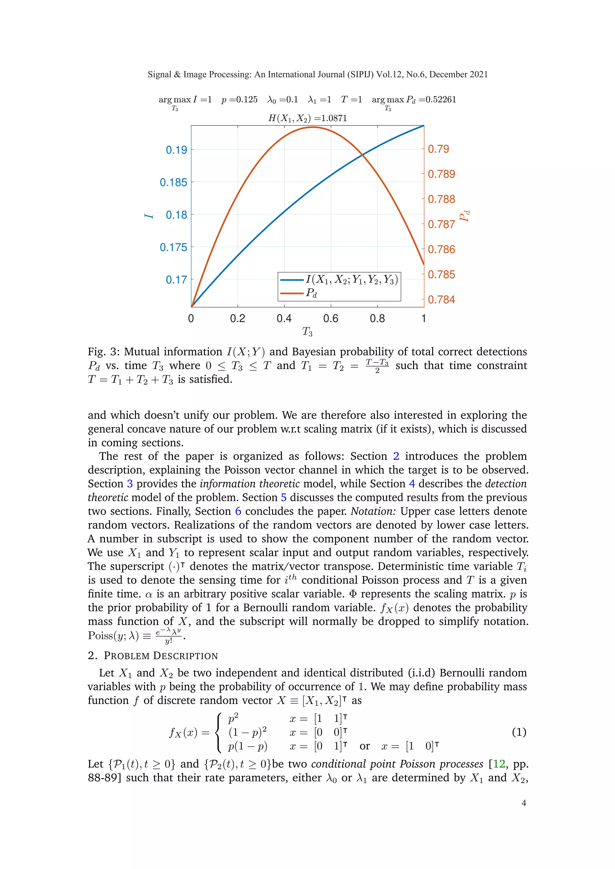
Fig. 3: Mutual information I(X; Y ) and Bayesian probability of total correct detections
Pd vs. time T3 where 0 ≤ T3 ≤ T and T1 = T2 = T −T3
2 such that time constraint
T = T1 + T2 + T3 is satisfied.
and which doesn’t unify our problem. We are therefore also interested in exploring the
general concave nature of our problem w.r.t scaling matrix (if it exists), which is discussed
in coming sections.
The rest of the paper is organized as follows: Section 2 introduces the problem
description, explaining the Poisson vector channel in which the target is to be observed.
Section 3 provides the information theoretic model, while Section 4 describes the detection
theoretic model of the problem. Section 5 discusses the computed results from the previous
two sections. Finally, Section 6 concludes the paper. Notation: Upper case letters denote
random vectors. Realizations of the random vectors are denoted by lower case letters.
A number in subscript is used to show the component number of the random vector.
We use X1 and Y1 to represent scalar input and output random variables, respectively.
The superscript (·)|
denotes the matrix/vector transpose. Deterministic time variable Ti
is used to denote the sensing time for ith
conditional Poisson process and T is a given
finite time. α is an arbitrary positive scalar variable. Φ represents the scaling matrix. p is
the prior probability of 1 for a Bernoulli random variable. fX(x) denotes the probability
mass function of X, and the subscript will normally be dropped to simplify notation.
Poiss(y; λ) ≡ e−λ
λy
y! .
2. PROBLEM DESCRIPTION
Let X1 and X2 be two independent and identical distributed (i.i.d) Bernoulli random
variables with p being the probability of occurrence of 1. We may define probability mass
function f of discrete random vector X ≡ [X1, X2]|
as
fX(x) =



p2
x = [1 1]|
(1 − p)2
x = [0 0]|
p(1 − p) x = [0 1]|
or x = [1 0]|
(1)
Let {P1(t), t ≥ 0} and {P2(t), t ≥ 0}be two conditional point Poisson processes [12, pp.
88-89] such that their rate parameters, either λ0 or λ1 are determined by X1 and X2,
Signal & Image Processing: An International Journal (SIPIJ) Vol.12, No.6, December 2021
4

8. respectively. That is, λ(xi) = λ0 if xi = 0 and λ1 if xi = 1, for i = 1, 2. λ0 and λ1 are
assumed known. We may count the number of arrivals from the two conditional Poisson
arrival processes in three possible configurations: two by individually counting the arrivals
from the two processes P1, P2 and one by counting the arrivals from the sum of two
processes {P1(t) + P2(t), t ≥ 0} with given rate parameter λ(X1) + λ(X2) as illustrated
in Figs.(1) and (2). The counting is performed such that at any given time, only one
of the three possible configurations is active. Furthermore, because of the independent
increments property of conditional Poisson processes, it is not necessary to switch back and
forth among possible configurations; it is sufficient to be in configuration 1 for time T1,
followed by configuration 2 for time T2, and then configuration 3 for time T3. Additionally,
counting is performed with a finite time constraint T = T1 + T2 + T3 where T1, T2 and
T3 are the unknown time proportions in counting arrivals from processes {P1(t), t ≥ 0},
{P2(t), t ≥ 0} and {P1(t) + P2(t), t ≥ 0}, respectively and T is total time. After utilizing
available time T, the above counting paradigm leads to a multivariate Poisson mixture
model with four component in three dimensions; we write random vector Y |
≡ [Y1 Y2 Y3],
so that Y ∈ {0, 1, 2, 3 · · · }3
. Each Yi is Poisson random variable given X; such that their
conditional law is,
Y1|X1 ∼ Poiss
y1; λ0 · (1 − X1) + λ1 · X1
· T1
Y2|X2 ∼ Poiss
y2; λ0 · (1 − X2) + λ1 · X2
· T2
Y3|(X1 + X2) ∼ Poiss
y3; (2 − (X1 + X2)) · λ0+
(X1 + X2) · λ1
· T3
. (2)
The observed random vector Y carries information about hidden random vector X|
≡
[X1 X2]. We are interested in strategies for selecting the times T1, T2, T3 that optimize
some cost related to the inference problem, either mutual information or probability
of correct detection. Strategies that involve setting T3 to 0 are referred to as individual
sensing; any time spent looking at combined counts is termed joint sensing. The general
case, which involves some individual and some joint sensing, will be referred to as hybrid
sensing.
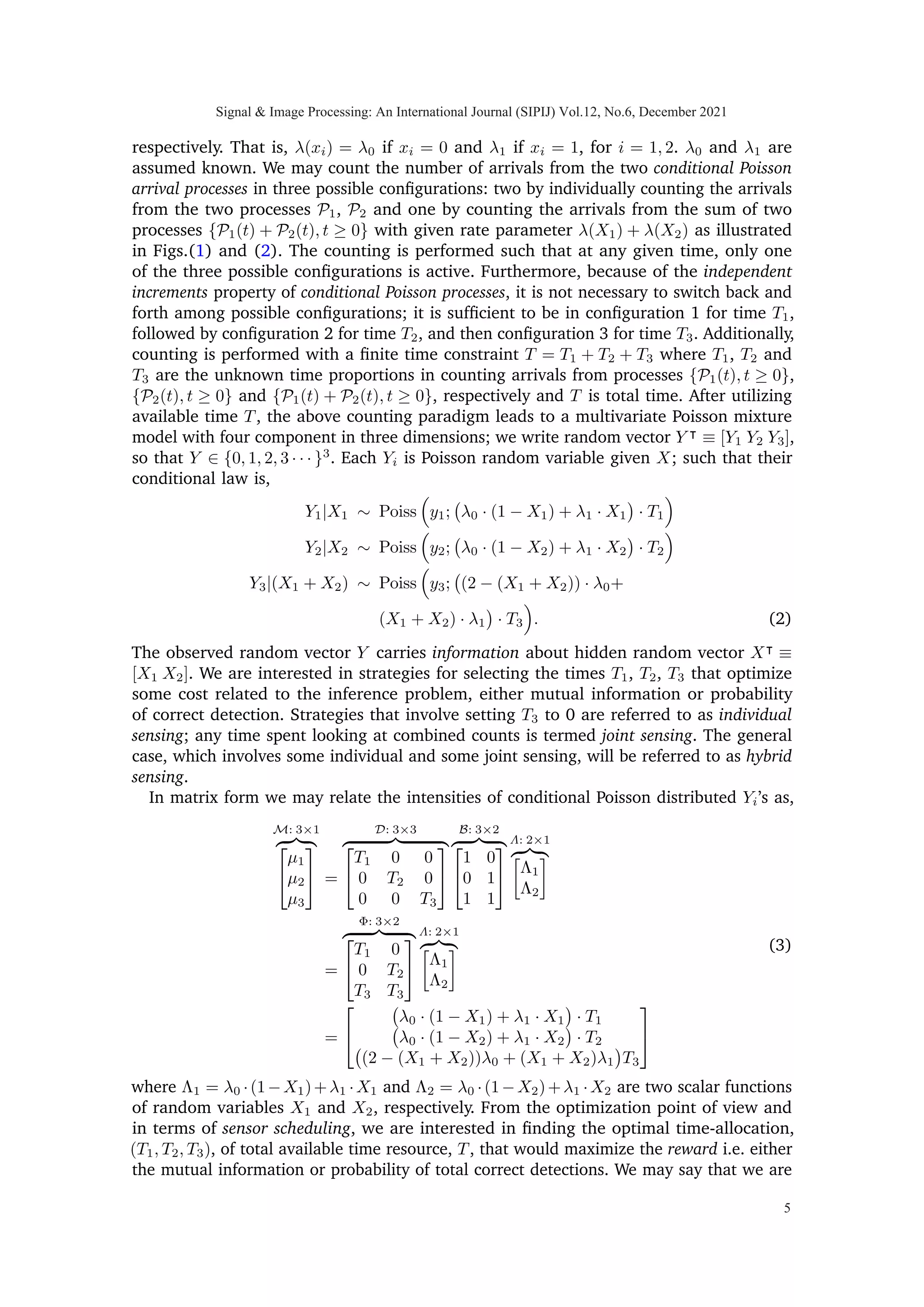
In matrix form we may relate the intensities of conditional Poisson distributed Yi’s as,
M: 3×1
z }| {


µ1
µ2
µ3

 =
D: 3×3
z }| {


T1 0 0
0 T2 0
0 0 T3


B: 3×2
z }| {


1 0
0 1
1 1


Λ: 2×1
z }| {
Λ1
Λ2
=
Φ: 3×2
z }| {


T1 0
0 T2
T3 T3


Λ: 2×1
z }| {
Λ1
Λ2
=


λ0 · (1 − X1) + λ1 · X1
· T1
λ0 · (1 − X2) + λ1 · X2
· T2
(2 − (X1 + X2))λ0 + (X1 + X2)λ1
T3


(3)
where Λ1 = λ0 ·(1−X1)+λ1 ·X1 and Λ2 = λ0 ·(1−X2)+λ1 ·X2 are two scalar functions
of random variables X1 and X2, respectively. From the optimization point of view and
in terms of sensor scheduling, we are interested in finding the optimal time-allocation,
(T1, T2, T3), of total available time resource, T, that would maximize the reward i.e. either
the mutual information or probability of total correct detections. We may say that we are
Signal Image Processing: An International Journal (SIPIJ) Vol.12, No.6, December 2021
5

9. 0 0.2 0.4 0.6 0.8 1
0
0.2
0.4
0.6
0.8
1
0.5
0.6
0.7
0.8
0.9
1
Fig. 4: Scalar Poisson channel: mutual information I(X1; Y1) and probability of total
correct detections Pd vs. time T.
interested in finding the diagonal matrix D, such that the mutual information I(X; Y ) is
maximized under time constraint T = T1 + T2 + T3. Configuration matrix B represents
all possible sensing combinations and Λ is the Poisson rate parameter vector. Vector M
is the vector of intensities of the Poisson random variables Y1, Y2, and Y3.
Mathematically we may write
max
T1,T2,T3
I(X1, X2; Y1, Y2, Y3) s.t. T1 + T2 + T3 = T. (4)
We may rewrite the objective function
max
T1,T2,T3
I(X1, X2; Y1, Y2, Y3) s.t. T1 + T + T3 = 1 (5)
where 0 ≤ T1 ≤ 1, 0 ≤ T2 ≤ 1 and 0 ≤ T3 ≤ 1. Without loss of generality we can take
T = 1 since the means of the observed Yi variables are the product of rate and time,
and any change in the total available time can be reflected in the rates, or equivalently
changing the time units.
We extend our understanding by looking at the same problem from the detection
theoretic aspect. For this, we maximize the Bayesian probability of total correct detection,
Pd, of hidden random vector X from observable random vector Y , as
max
T1,T2,T3
Pd s.t. T1 + T2 + T3 = 1 (6)
and compare the results to formerly computed information theoretic results. Simulations
on empirical data are performed by varying different parameters involved in the model
for further validation of computed results.
3. INFORMATION THEORETIC DESCRIPTION
A. Scalar Poisson channel
Firstly the scalar version of the Poisson channel is presented and then it is extended to
the vector version of our problem. We start with mutual information between a scalar
Signal Image Processing: An International Journal (SIPIJ) Vol.12, No.6, December 2021
6

10. Bernoulli random variable X1 and Y1 which is a scalar and two component Poisson
mixture. The probability mass function of Y1 is then given as
f(y1) = (1 − p) · Poiss(y1; Tλ0) + p · Poiss(y1; Tλ1).
The mutual information I can be written as
I(X1; Y1) = H(Y1) − H(Y1|X1)
where H(·) is the Shannon entropy, which is defined as a discrete functional H : f →
−
P
Y ∈Y
f · log2(f) and f is the probability mass function of random variate Y with Y as
the corresponding support. We may write H(Y1) as
H(Y1) = −
∞
X
y1=0
[(1 − p) · Poiss(y1; Tλ0) + p
· Poiss(y1; Tλ1)] · log2[(1 − p) · Poiss(y1; Tλ0)
+ p · Poiss(y1; Tλ1)]
,
and
H(Y1|X1) =
X
x1∈X1
f(x1)
∞
X
y1=0
−f(y1|x1) · log2[f(y1|x1)]
= −
(1 − p)
∞
X
y1=0
Poiss(y1; Tλ0)
· log2[Poiss(y1; Tλ0)] + p
∞
X
y1=0
Poiss(y1; Tλ1)
· log2[Poiss(y1; Tλ1)]
.
In Fig. (4), for a scalar Poisson channel discussed above, I(X1; Y1) and Pd illustrates a
monotonic relationship w.r.t T, as expected.
B. Vector Poisson channel
Mutual information between two random vectors can be defined as the difference
between the total entropy in one random vector and the conditional entropy in the second
random vector given the first vector. We write
I(X; Y ) = H(Y ) − H(Y |X) (7)
The conditional entropy H(Y |X) is calculated from the conditional probability mass
functions f(y|X = [x1 x2]|
) defined as
f(y|X = [0 0]|
)
= Poiss(y1; λ0T1) · Poiss(y2; λ0T2) · Poiss(y3; 2λ0T3),
f(y|X = [0 1]|
)
= Poiss(y1; λ0T1) · Poiss(y2; λ1T2) · Poiss(y3; (λ0 + λ1)T3),
f(y|X = [1 0]|
)
= Poiss(y1; λ1T1) · Poiss(y2; λ0T2) · Poiss(y3; (λ1 + λ0)T3),
f(y|X = [1 1]|
)
= Poiss(y1; λ1T1) · Poiss(y2; λ1T2) · Poiss(y3; 2λ1T3).
Signal Image Processing: An International Journal (SIPIJ) Vol.12, No.6, December 2021
7

11. The marginal probability mass function of Y is then given as
f(y)
= (1 − p)2
· f(y|X = [0 0]|
) + p(1 − p)·
f(y|X = [0 1]|
) + p(1 − p) · f(y|X = [1 0]|
)+
p2
· f(y|X = [1 1]|
). (8)
Using the identity defined in (7) and the definition of entropy defined above, the mutual
information I(X; Y ) becomes
I(X; Y )
=
∞
X
y1=0
∞
X
y2=0
∞
X
y3=0
−f(y1, y2, y3) · log2[f(y1, y2, y3)])
−
X
X∈X
f(x)
h ∞
X
y1=0
∞
X
y2=0
∞
X
y3=0
−f(y1, y2, y3|X)
· log2[f(y1, y2, y3|X)]
i
. (9)
A complete expression for mutual information is given in Appendix A.
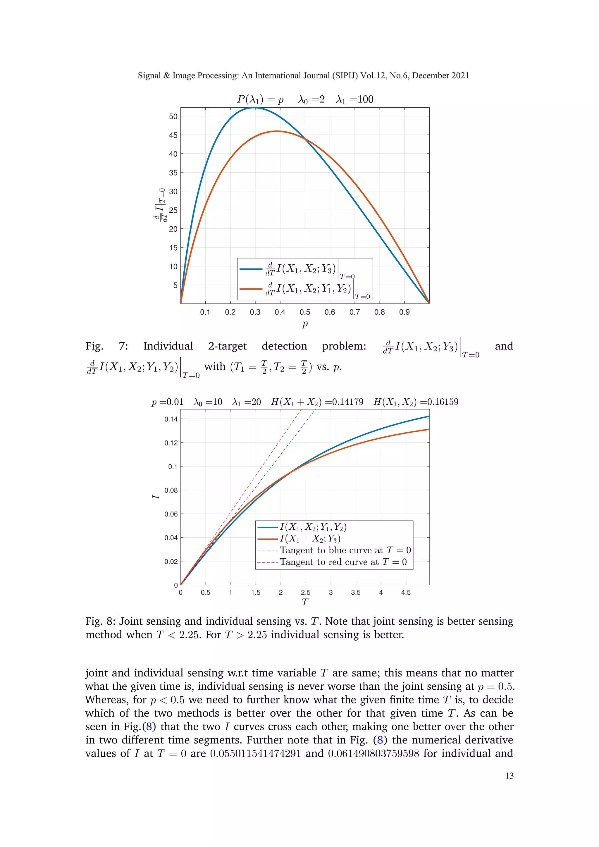
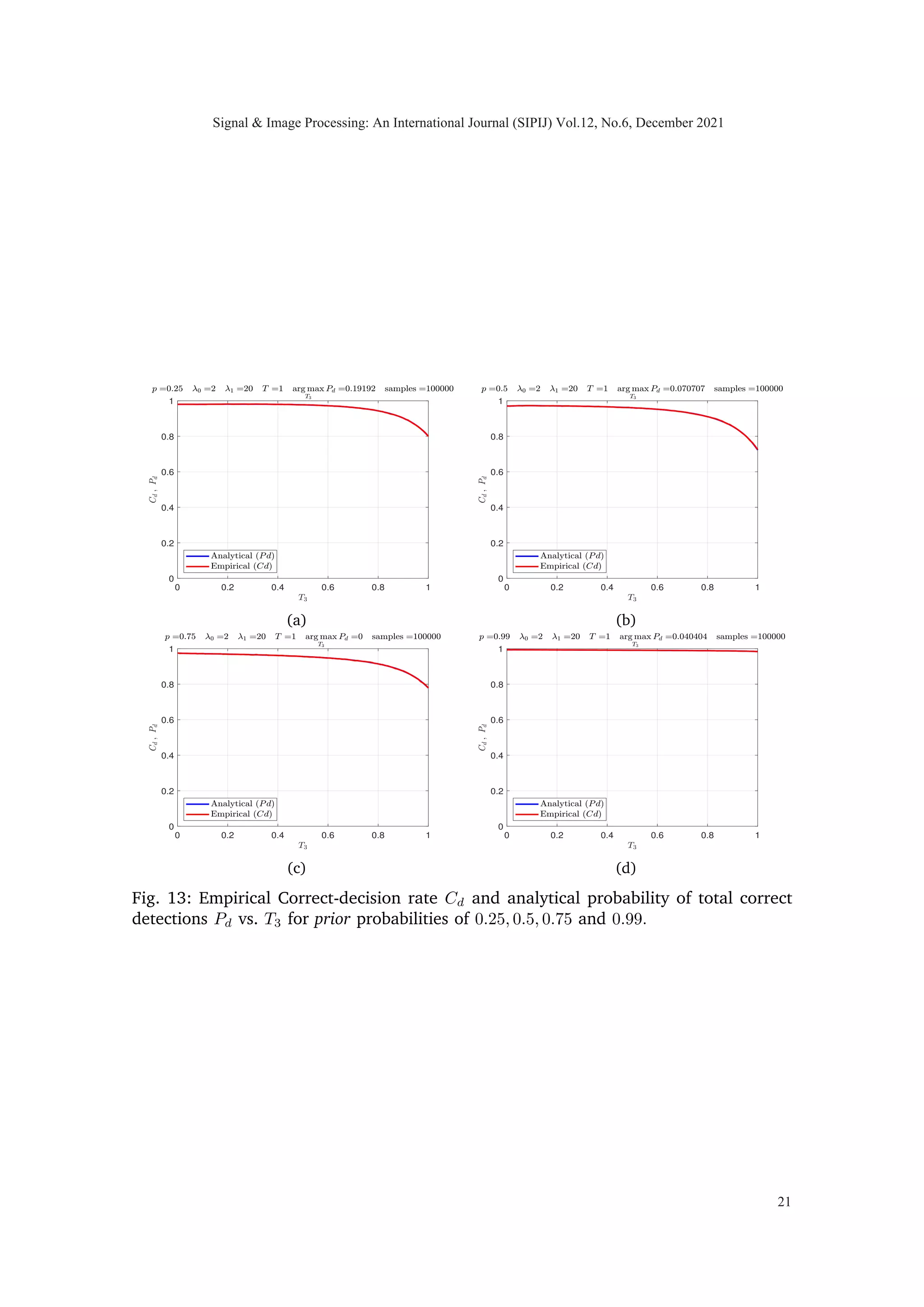
Fig. (3) illustrates the concavity of mutual information as a function of T3 (constrained
problem), in a vector Poisson channel defined in (2) and illustrated in Fig. (1), when
three sensing times are varied according to (T1, T2, T3) = (1−T3
2 , 1−T3
2 , T3) and 0 ≤ T3 ≤ 1.
It can also be seen that the two metrics Pd and I are maximizing at two different input
argument values.
Theorem 1: I(X1, X2; Y1, Y2, Y3) is concave in T3 = 0 plane.
Proof:
I(X1, X2; Y1, Y2, Y3)

14. T3=0
= I(X1, X2; Y1, Y2)
By chain rule of mutual information:
I(X1, X2; Y1, Y2) = I(X1, X2; Y1) + I(X1, X2; Y2|Y1)
=I(X1; Y1) + I(X2; Y2). (10)
We note in (10) that each I(Xi; Yi) is solely a function of Ti and also concave in it [9,
p. 1306][13]. We further know that sum of concave functions is a concave function.
Therefore I(X1, X2; Y1, Y2) is concave in T1 and T2 when T3 = 0. This concludes the
proof.
Theorem 2: I(X1, X2; Y1, Y2, Y3) is symmetric in variables T1 and T2.
Proof: Mutual information I(X1, X2; Y1, Y2, Y3) given in appendix A is invariant under
any permutation of variables T1 and T2. That means interchanging the two variables
leaves the expression unchanged.
If we further expand the expression for mutual information between X and Y using
chain rule [14] [15] as,
I(X1, X2; Y1, Y2, Y3)
= I(X1, X2; Y1) + I(X1, X2; Y2|Y1) + I(X1, X2; Y3|Y1, Y2)
= I(X1; Y1) +
0
z }| {
I(X2; Y1|X1) +
0
z }| {
I(X1; Y2|Y1) +
I(X2;Y2)
z }| {
I(X2; Y2|Y1, X1) +I(X1, X2; Y3|Y1, Y2)
= I(X1; Y1) + I(X2; Y2) + I(X1, X2; Y3|Y1, Y2). (11)
Signal Image Processing: An International Journal (SIPIJ) Vol.12, No.6, December 2021
8

15. 0 0.2 0.4 0.6 0.8 1
0
0.2
0.4
0.6
0.8
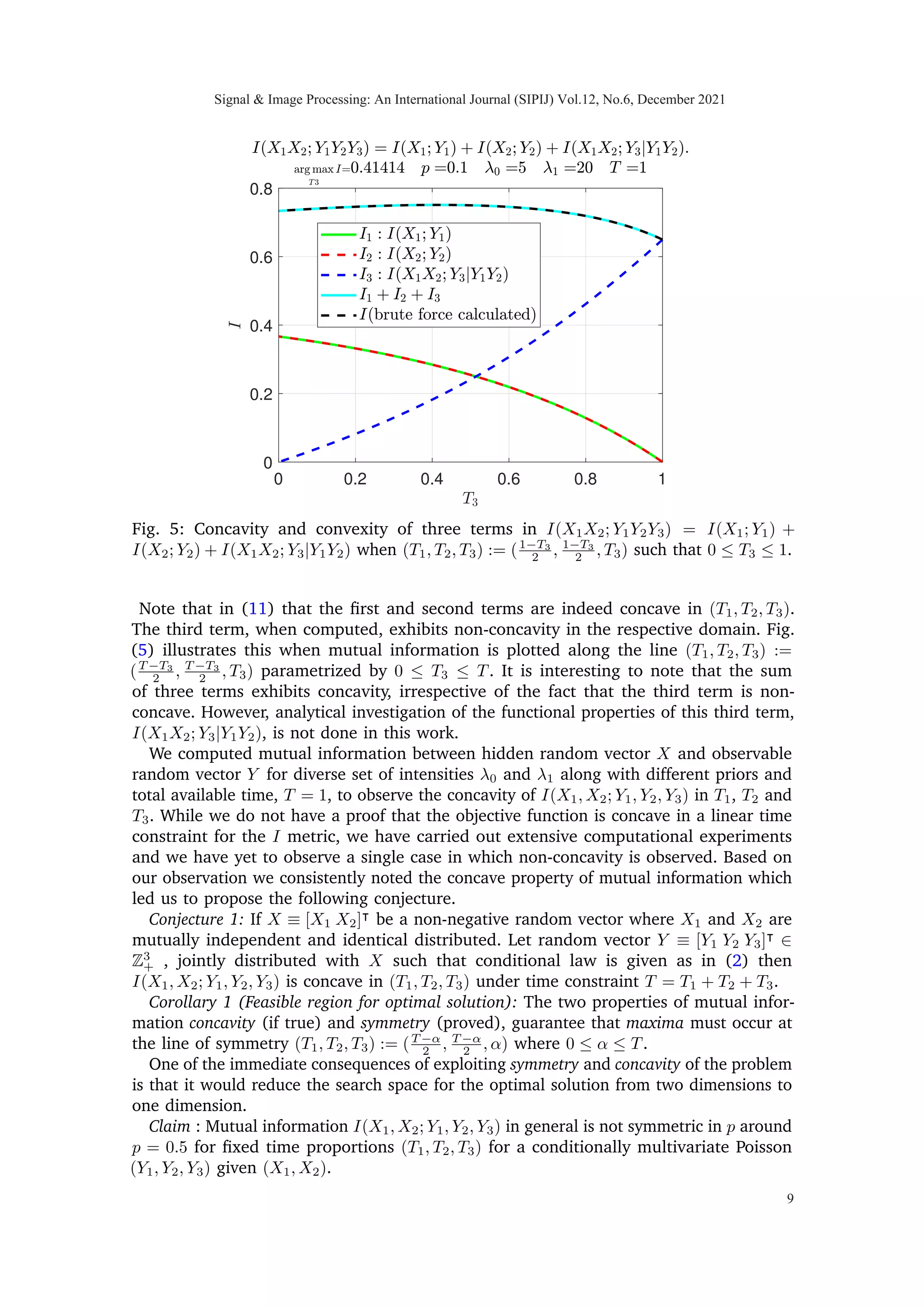
Fig. 5: Concavity and convexity of three terms in I(X1X2; Y1Y2Y3) = I(X1; Y1) +
I(X2; Y2) + I(X1X2; Y3|Y1Y2) when (T1, T2, T3) := (1−T3
2 , 1−T3
2 , T3) such that 0 ≤ T3 ≤ 1.
Note that in (11) that the first and second terms are indeed concave in (T1, T2, T3).
The third term, when computed, exhibits non-concavity in the respective domain. Fig.
(5) illustrates this when mutual information is plotted along the line (T1, T2, T3) :=
(T −T3
2 , T −T3
2 , T3) parametrized by 0 ≤ T3 ≤ T. It is interesting to note that the sum
of three terms exhibits concavity, irrespective of the fact that the third term is non-
concave. However, analytical investigation of the functional properties of this third term,
I(X1X2; Y3|Y1Y2), is not done in this work.
We computed mutual information between hidden random vector X and observable
random vector Y for diverse set of intensities λ0 and λ1 along with different priors and
total available time, T = 1, to observe the concavity of I(X1, X2; Y1, Y2, Y3) in T1, T2 and
T3. While we do not have a proof that the objective function is concave in a linear time
constraint for the I metric, we have carried out extensive computational experiments
and we have yet to observe a single case in which non-concavity is observed. Based on
our observation we consistently noted the concave property of mutual information which
led us to propose the following conjecture.
Conjecture 1: If X ≡ [X1 X2]|
be a non-negative random vector where X1 and X2 are
mutually independent and identical distributed. Let random vector Y ≡ [Y1 Y2 Y3]|
∈
Z3
+ , jointly distributed with X such that conditional law is given as in (2) then
I(X1, X2; Y1, Y2, Y3) is concave in (T1, T2, T3) under time constraint T = T1 + T2 + T3.
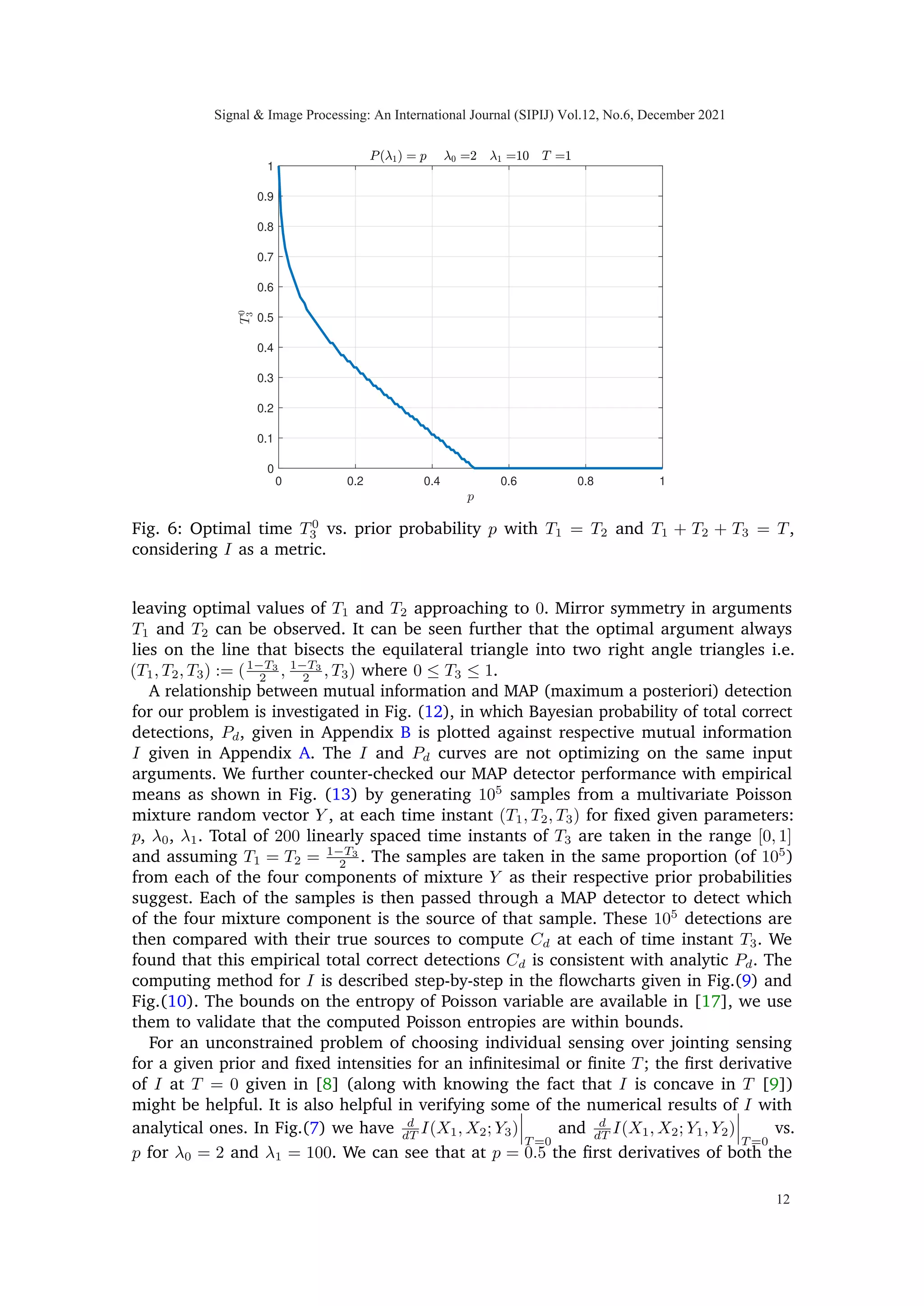
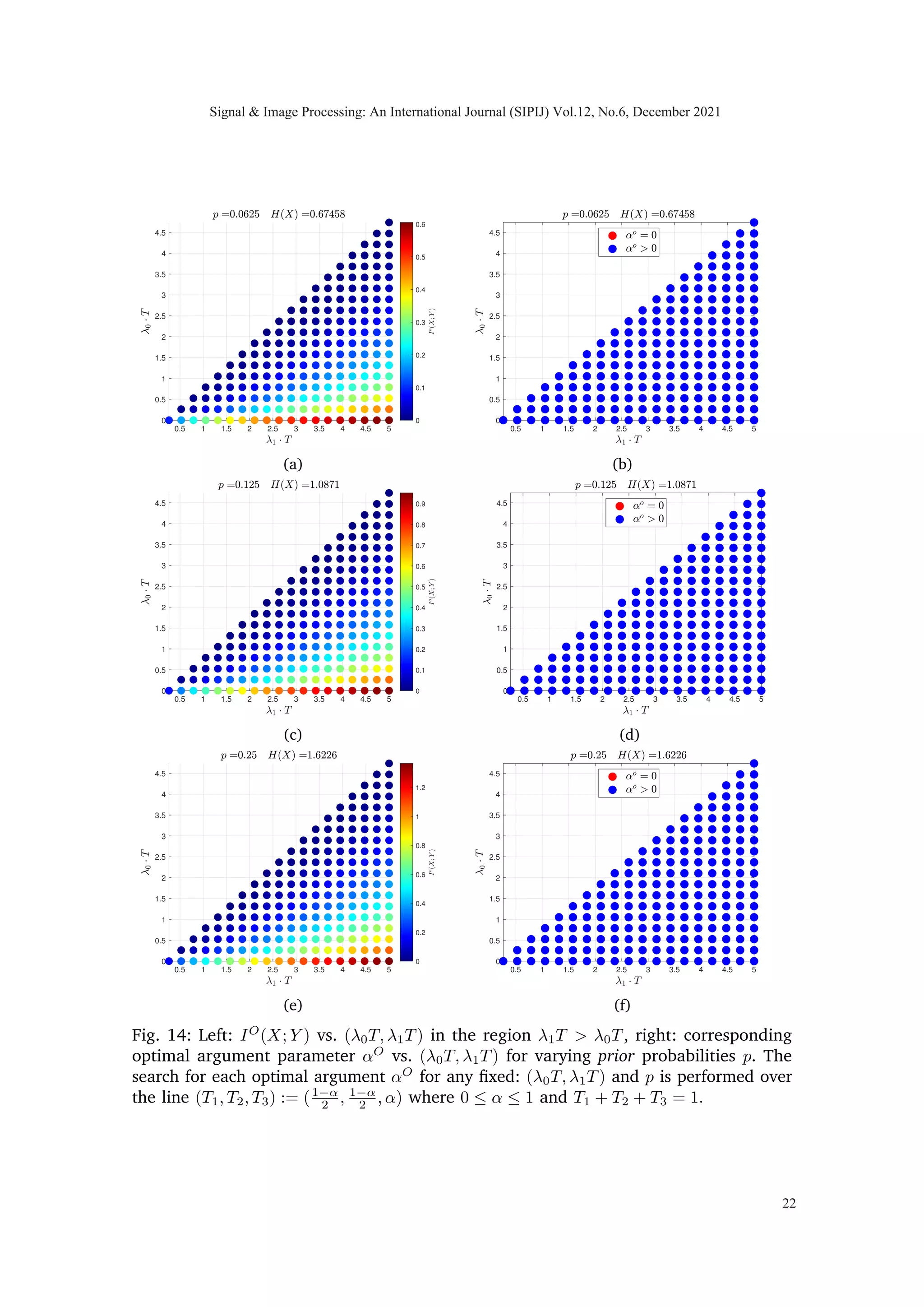
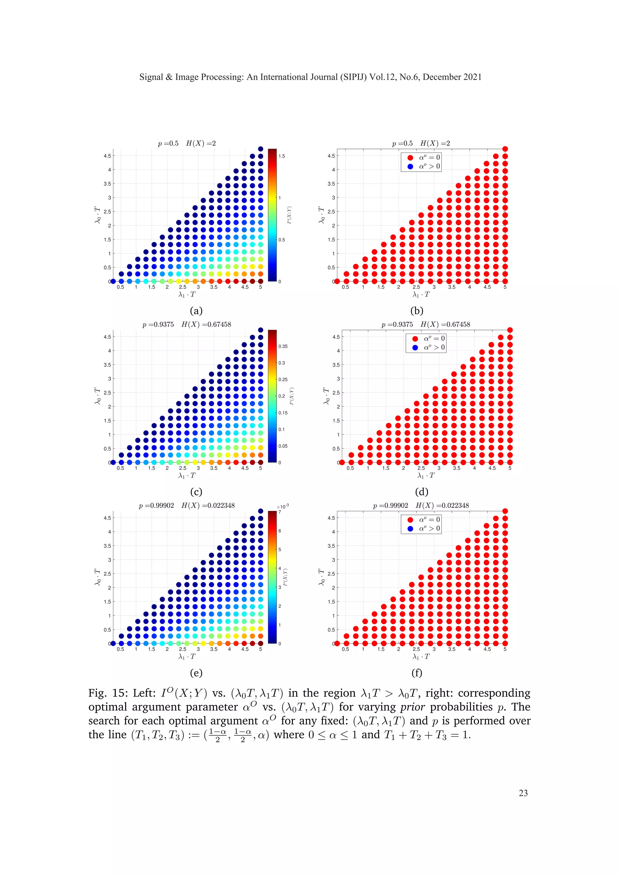
Corollary 1 (Feasible region for optimal solution): The two properties of mutual infor-
mation concavity (if true) and symmetry (proved), guarantee that maxima must occur at
the line of symmetry (T1, T2, T3) := (T −α
2 , T −α
2 , α) where 0 ≤ α ≤ T.
One of the immediate consequences of exploiting symmetry and concavity of the problem
is that it would reduce the search space for the optimal solution from two dimensions to
one dimension.
Claim : Mutual information I(X1, X2; Y1, Y2, Y3) in general is not symmetric in p around
p = 0.5 for fixed time proportions (T1, T2, T3) for a conditionally multivariate Poisson
(Y1, Y2, Y3) given (X1, X2).
Signal Image Processing: An International Journal (SIPIJ) Vol.12, No.6, December 2021
9

16. Example: For a scalar random variable X1 and conditional Poisson variable Y1 with
scaling factor T, we have equation (115) on page (10) of [8], given below
d
dT
I(X1; Y1)

19. T =0
= E[Λ1 · log Λ1] − E[Λ1] · log(E[Λ1]).
(12)
where Λ1 = λ0 ·(1−X1)+λ1 ·X1. When we consider a random vector X (instead of scalar
random variable as above), and take distribution on X as given in (1). Dividing variable
total time T equally in counting arrivals from X1 and X2 separately: T1 = T2 = T
2 and
T3 = 0, we have
I(X1, X2; Y1, Y2, Y3)

22. T1= T
2 ,T2= T
2 ,T3=0
=
2 · I(X1; Y1)

25. T1= T
2
(13)
Let T be a free variable in (13), we have
d
dT
I(X1, X2; Y1, Y2, Y3)

28. T1= T
2 ,T2= T
2 ,T3=0
!

33. T =0
=
(1 − p) · λ0 · log2(λ0) + p · λ1 · log2(λ1)−
(1 − p) · λ0 + p · λ1
· log2
(1 − p) · λ0 + p · λ1
(14)
Equation (14) is concave in p
d2
dp2
d
dT
I(X1, X2; Y1, Y2, Y3)

36. T1= T
2 ,T2= T
2 ,T3=0

41. T =0
!
= −
(λ0 − λ1)2
Ln(2) · (1 − p)λ0 + p · λ1
0 (15)
Maxima of equation (14) occurs at p = 4−e
e when λ0 = 2 and λ1 = 4. Since (14) is
concave in p, then if it was symmetric, maxima must had occurred at p = 0.5.
4. DETECTION THEORETIC DESCRIPTION
A. Maximization of probability of total correct detections in sensing time intervals
In previous section, we discussed and presented the metric of mutual information
I between hidden random vector X, and observable vector Y . Here we approach the
original sensing problem as a multi-hypothesis detection problem and find the optimal
solution by minimizing the Bayesian risk [16, pp.220] in sensing times i-e (T1, T2, T3).
We define Bayes risk r as
r = (1 − p)2
h
P00 | 00 C00 | 00 + P01 | 00 C01 | 00
+P10 | 00 C10 | 00 + P11 | 00 C11 | 00
i
+ p(1 − p)
h
P00 | 01 C00 | 01 + P01 | 01 C01 | 01 + P10 | 01 C10 | 01
+P11 | 01 C11 | 01
i
+ p(1 − p)
h
P00 | 10 C00 | 10
+P01 | 10 C01 | 10 + P10 | 10 C10 | 10 + P11 | 10 C11 | 10
i
+p2
h
P00 | 11 C00 | 11 + P01 | 11 C01 | 11 + P10 | 11 C10 | 11
+P11 | 11 C11 | 11
i
,
Signal Image Processing: An International Journal (SIPIJ) Vol.12, No.6, December 2021
10

42. where Pkl | ij is the probability that X = [xi
1 xj
2]|
is true while decision X = [xk
1 xl
2]|
is made; similarly for Ckl | ij. Setting all costs for which [xi
1 xj
2]|
6= [xk
1 xl
2]|
to one and
[xi
1 xj
2]|
= [xk
1 xl
2]|
to zero, we have
r = (1 − p)2
h
P01 | 00 + P10 | 00 + P11 | 00
i
+ p(1 − p)
h
P00 | 01 + P10 | 01 + P11 | 01
i
+ p(1 − p)
h
P00 | 10 + P01 | 10 + P11 | 10
i
+ p2
h
P00 | 11 + P01 | 11 + P10 | 11
i
. (16)
We are interested in minimizing this Bayes risk r in (T1, T2, T3) i-e
min
T1,T2,T3
r s.t. T1 + T2 + T3 = 1. (17)
Note that while minimizing r in (T1, T2, T3), the decisions boundaries would be changing
accordingly and become function of (T1, T2, T3). Equivalently, we may say that
max
T1,T2,T3
Pd s.t. T1 + T2 + T3 = 1 (18)
where Pd is probability of total correct detections, Pd = 1 − r. In the next section
we compute I ans Pd, for different channel parameters, given in Appendices A and B,
respectively.
5. COMPUTATIONAL AND SIMULATION RESULTS
The primary purpose of performing the computations and simulations is twofold: the
first is to see under what circumstances which of the sensing method: individual, joint or
hybrid sensing is optimal since analytical solutions for the two objective functions do
not exist; and the second is to investigate whether the two metrics I and Pd leads to
the same or different maximizing input arguments. The objective function, defined in
(4) is observed to be a convex optimization problem when a pre-defined channel scaling
matrix structure is imposed. For all computational purposes, we always approximate the
Poisson mass function by truncating it; truncation is done by a rectangular window that
extends from lower limit 0 to the upper limit where Poisson pmf drops in value below
double precision machine epsilon ( = 2−53
) as given in Appendix C.
Fig. (6) illustrates how the optimal input argument T3 moves from 0 to 1 as prior
0 p 1 is varied while input intensities are held fixed. Ninety linearly spaced discrete
points in the range (0, 0.5] are first taken for prior p and then another ten linearly spaced
points are taken in the interval (0.5, 1), constituting a total of hundred points of p for
computations. For every value of prior p; another hundred linearly spaced points for
time proportion T3 are taken in the closed interval [0, 1] such that T1 = T2 = 1−T3
2 and
T1 + T2 + T3 = 1. At every instant of p, hundred values of I are computed corresponding
to hundred time proportion. Maximum value of I is then sought and the corresponding
value of T3 is plotted against prior p. The plot signifies that if the prior p is closer to 0
then all time T be invested in joint sensing whereas as prior increases from 0 towards 1,
individual sensing progressively starts to take more and more proportion of total available
time T. This phenomena is further explored in scatter plots where input intensities are
varied too.
In Fig. (11), ternary plots of I are shown as prior p is varied. The vertices of the
equilateral triangle are at (T1, 0, 0), (0, T2, 0) and (0, 0, T3) with T1 + T2 + T3 = 1. It
can be seen that the distribution of time resource T = 1 changes as p is varied. As p
tends to 0, the optimal value of T3 tends to consume all the available time resource T
Signal Image Processing: An International Journal (SIPIJ) Vol.12, No.6, December 2021
11

43. 0 0.2 0.4 0.6 0.8 1
0
0.1
0.2
0.3
0.4
0.5
0.6
0.7
0.8
0.9
1
Fig. 6: Optimal time T0
3 vs. prior probability p with T1 = T2 and T1 + T2 + T3 = T,
considering I as a metric.
leaving optimal values of T1 and T2 approaching to 0. Mirror symmetry in arguments
T1 and T2 can be observed. It can be seen further that the optimal argument always
lies on the line that bisects the equilateral triangle into two right angle triangles i.e.
(T1, T2, T3) := (1−T3
2 , 1−T3
2 , T3) where 0 ≤ T3 ≤ 1.
A relationship between mutual information and MAP (maximum a posteriori) detection
for our problem is investigated in Fig. (12), in which Bayesian probability of total correct
detections, Pd, given in Appendix B is plotted against respective mutual information
I given in Appendix A. The I and Pd curves are not optimizing on the same input
arguments. We further counter-checked our MAP detector performance with empirical
means as shown in Fig. (13) by generating 105
samples from a multivariate Poisson
mixture random vector Y , at each time instant (T1, T2, T3) for fixed given parameters:
p, λ0, λ1. Total of 200 linearly spaced time instants of T3 are taken in the range [0, 1]
and assuming T1 = T2 = 1−T3
2 . The samples are taken in the same proportion (of 105
)
from each of the four components of mixture Y as their respective prior probabilities
suggest. Each of the samples is then passed through a MAP detector to detect which
of the four mixture component is the source of that sample. These 105
detections are
then compared with their true sources to compute Cd at each of time instant T3. We
found that this empirical total correct detections Cd is consistent with analytic Pd. The
computing method for I is described step-by-step in the flowcharts given in Fig.(9) and
Fig.(10). The bounds on the entropy of Poisson variable are available in [17], we use
them to validate that the computed Poisson entropies are within bounds.
For an unconstrained problem of choosing individual sensing over jointing sensing
for a given prior and fixed intensities for an infinitesimal or finite T; the first derivative
of I at T = 0 given in [8] (along with knowing the fact that I is concave in T [9])
might be helpful. It is also helpful in verifying some of the numerical results of I with
analytical ones. In Fig.(7) we have d
dT I(X1, X2; Y3)

46. T =0
and d
dT I(X1, X2; Y1, Y2)

49. T =0
vs.
p for λ0 = 2 and λ1 = 100. We can see that at p = 0.5 the first derivatives of both the
Signal Image Processing: An International Journal (SIPIJ) Vol.12, No.6, December 2021
12

50. 0.1 0.2 0.3 0.4 0.5 0.6 0.7 0.8 0.9
5
10
15
20
25
30
35
40
45
50
Fig. 7: Individual 2-target detection problem: d
dT I(X1, X2; Y3)

53. T =0
and
d
dT I(X1, X2; Y1, Y2)

56. T =0
with (T1 = T
2 , T2 = T
2 ) vs. p.
0 0.5 1 1.5 2 2.5 3 3.5 4 4.5
0
0.02
0.04
0.06
0.08
0.1
0.12
0.14
Fig. 8: Joint sensing and individual sensing vs. T. Note that joint sensing is better sensing
method when T 2.25. For T 2.25 individual sensing is better.
joint and individual sensing w.r.t time variable T are same; this means that no matter
what the given time is, individual sensing is never worse than the joint sensing at p = 0.5.
Whereas, for p 0.5 we need to further know what the given finite time T is, to decide
which of the two methods is better over the other for that given time T. As can be
seen in Fig.(8) that the two I curves cross each other, making one better over the other
in two different time segments. Further note that in Fig. (8) the numerical derivative
values of I at T = 0 are 0.055011541474291 and 0.061490803759598 for individual and
Signal Image Processing: An International Journal (SIPIJ) Vol.12, No.6, December 2021
13

57. joint sensing, respectively when I is computed according to the algorithm defined in
flowcharts. Now compare these numerical derivative values with analytically calculated
ones 0.055011540931595 and 0.061490807291534; the two are accurate to eight decimal
places, this validates that computations are accurate enough.
Fig. (14) and Fig. (15) illustrates the scatter plots, for a range of varying input intensities
in constrained problem w.r.t I metric. The scatter plots on the left hand side illustrates the
optimal value of mutual information at any point (λ0 · T, λ1 · T) where λ0 · T λ1 · T and
0 λ1 · T ≤ 5 for a given prior p and T = 1. The corresponding maximizing argument
is shown on the left hand side of the scatter plots. It is noticed that for prior p 0.5,
farther the four components of multivariate mixture Poisson are from each other in terms
of their intensities; more the optimal solution moves towards the individual sensing. In
other words if the four pmfs (under hypothesis testing) gets closer, more the optimal
sensing relies on joint sensing for prior p 0.5. If the prior p ≥ 0.5 then irrespective of
the other parameter values in the model, individual sensing is the optimal strategy from
I metric.
6. CONCLUSION
In this work we have addressed a simple abstract sensor scheduling problem in which
two Poisson sources are observed either individually or jointly with a switching mechanism
and a single counter. The scheduling problem is to choose the times associated with the
different switch configurations given a total time constraint.
For our specific problem we were able to solve the optimization problem using compu-
tational methods, primarily because of the relatively small number of free parameters. For
the case in which mutual information is the cost function, we observed but were unable
to prove that the cost function is concave in the switch times; if true this reduces the
optimization problem to a one-dimensional search. We observed that the two different
metrics of mutual information and probability of correct detection did not always lead to
the same scheduling solution. A second interesting result was that, under the mutual
information metric, when the prior p on the sources was greater than 0.5, individual
sensing was always the best that could be done.
In a certain sense our computational results are not particularly interesting. In most cases
the cost functions are quite flat and there were no dramatic variation in mutual information
or probability of correct detection across the space of possible switch configuration times.
A communications engineer faced with the problem exactly as we have posed it would be
hard-pressed to justify doing anything other than the simplest and most obvious solution,
namely taking the available time and dividing it equally between individual observation
of the two sources.
However, the fact that there is some variation in performance based in intelligent choice
of the switch times leaves open the possibility of the value of investigations like ours for
more complex problems. Several extensions immediately come to mind: more sources
(perhaps hundreds or thousands, not two), unknown Poisson rates, different unknown
or nonexistent priors, different source distributions. Unfortunately, the jump to a larger
number of sources brings with it a combinatorial explosion which would rule out the
brute-force optimization techniques used in this paper in very short order. Alternate
switching strategies might include an adaptive one in which the switching time and
configurations are determined online or in real time depending on the observations up
to the current time. We recommend and are interested in continuing investigations along
these lines.
Signal Image Processing: An International Journal (SIPIJ) Vol.12, No.6, December 2021
14

58. APPENDIX A
EXPRESSION OF MUTUAL INFORMATION I(X1, X2; Y1, Y2, Y3)
I(X; Y ) = −
∞
X
y1=0
∞
X
y2=0
∞
X
y3=0
(1 − p)2
· Poiss(y1; λ0T1) · Poiss(y2; λ0T2)·
Poiss(y3; 2λ0T3) + p(1 − p) · Poiss(y1; λ0T1) · Poiss(y2; λ1T2) · Poiss(y3; (λ0 + λ1)T3)+
p(1 − p) · Poiss(y1; λ1T1) · Poiss(y2; λ0T2) · Poiss(y3; (λ1 + λ0)T3) + p2
· Poiss(y1; λ1T1)·
Poiss(y2; λ1T2) · Poiss(y3; 2λ1T3)
!
· log2[(1 − p)2
· Poiss(y1; λ0T1) · Poiss(y2; λ0T2)·
Poiss(y3; 2λ0T3) + p(1 − p) · Poiss(y1; λ0T1) · Poiss(y2; λ1T2) · Poiss(y3; (λ0 + λ1)T3)+
p(1 − p) · Poiss(y1; λ1T1) · Poiss(y2; λ0T2) · Poiss(y3; (λ1 + λ0)T3)+
p2
· Poiss(y1; λ1T1) · Poiss(y2; λ1T2) · Poiss(y3; 2λ1T3)]
!#
+
(1 − p)2
·
∞
X
y1=0
∞
X
y2=0
∞
X
y3=0
(Poiss(y1; λ0T1) · Poiss(y2; λ0T2) · Poiss(y3; 2λ0T3))·
log2[Poiss(y1; λ0T1) · Poiss(y2; λ0T2) · Poiss(y3; 2λ0T3)]
!
+
p(1 − p) ·
∞
X
y1=0
∞
X
y2=0
∞
X
y3=0
(Poiss(y1; λ0T1) · Poiss(y2; λ1T2) · Poiss(y3; (λ0 + λ1)T3)·
log2[Poiss(y1; λ0T1) · Poiss(y2; λ1T2) · Poiss(y3; (λ0 + λ1)T3)]
!
+ p(1 − p)·
∞
X
y1=0
∞
X
y2=0
∞
X
y3=0
(Poiss(y1; λ1T1) · Poiss(y2; λ0T2) · Poiss(y3; (λ1 + λ0)T3)·
log2[Poiss(y1; λ1T1) · Poiss(y2; λ0T2) · Poiss(y3; (λ1 + λ0)T3)]
!
+
p2
·
∞
X
y1=0
∞
X
y2=0
∞
X
y3=0
(Poiss(y1; λ1T1) · Poiss(y2; λ1T2) · Poiss(y3; 2λ1T3)·
log2[(Poiss(y1; λ1T1) · Poiss(y2; λ1T2) · Poiss(y3; 2λ1T3)]
!#
.
Signal Image Processing: An International Journal (SIPIJ) Vol.12, No.6, December 2021
15

59. APPENDIX B
EXPRESSION OF PROBABILITY OF TOTAL CORRECT DETECTIONS Pd
Pd =
X
(y1,y2,y3)
f00 : {(f00 = f01) (f00 = f10) (f00 = f11)}+
X
(y1,y2,y3)
f01 : {(f01 f00) (f01 = f10) (f01 = f11))}+
X
(y1,y2,y3)
f10 : {(f10 f00) (f10 f01) (f10 = f11)}+
X
(y1,y2,y3)
f11 : {(f11 f00) (f11 f01) (f11 f10)}.
Where
f00 ≡ (1 − p)2
· Poiss(y1; λ0T1) · Poiss(y2; λ0T2) · Poiss(y3; 2λ0T3),
f01 ≡ p(1 − p) · Poiss(y1; λ0T1) · Poiss(y2; λ1T2) · Poiss(y3; (λ0 + λ1)T3),
f10 ≡ p(1 − p) · Poiss(y1; λ1T1) · Poiss(y2; λ0T2) · Poiss(y3; (λ1 + λ0)T3),
f11 ≡ p2
· Poiss(y1; λ1T1) · Poiss(y2; λ1T2) · Poiss(y3; 2λ1T3),
: logical AND operation
APPENDIX C
NUMERICAL APPROXIMATION OF THE POISSON PMF AND MUTUAL INFORMATION
Poiss(x; λ) ≈
eλ
λx
x! x ≤ xc
0 x xc
(19)
where xc is such that cummulative distribution function of Poisson random variable at
xc is approximately equal to 1. i.e. CDFPoiss(xc; λ) ≈ 1. When represented in double
precision floating-point arithmetic in IEEE 754 standard; this means that numerical values
of CDFPoiss(xc; λ) and CDFPoiss(xc + 1; λ) are identical and equal to numerical one.
The infinite summations in mutual information expression given in appendix A are all
truncated from 0 to xc = CDFPoiss−1
(1 − ; (λ1 + λ1)T) for a given value of λ1 and T.
CDFPoiss−1
is inverse Poisson cdf and is, the machine precision number, 2−53
[18].
APPENDIX D
CODE DESCRIPTION
Since computations for I can be done in parallel, we may exploit this fact by vector-
ization of the algorithm and then evaulating I at grid points in parallel as defined in
flowchart in Fig.(9) and Fig.(10) for fast computational throughput. However, it must
be noted that this way of vectorized computations by first performing the truncation
of Poisson distribution and then forming the grid of points, for further calculation of
I, is not effective for large values of Poisson intensities involved in the problem. This
is because the grid size increases cubely w.r.t truncated support of involved pmfs. So,
for large values of Poisson intensities, say λ 100, we need to resort to Monte Carlo
method.
For calculation of Pd, the same computed conditional Poisson pmfs can be used for all
the comparisons that are required in conditional expression given in Appendix B.
Signal Image Processing: An International Journal (SIPIJ) Vol.12, No.6, December 2021
16

60. Start
input variables
, , T
λ1 λ0
i D?
take D no. of points from convex set
{ + + = T :
T1 T2 T3
= , 0 ≤ ≤ , 0 ≤ ≤ T }
T1 T2 T1
T
2
T3
choose N no. of points from set
{p : 0 p 1}
collect (i, j value of
)
th
I ( ; )
X1X2 Y1Y2Y3
i := 1
j N ?
i := i + 1
True
False
End
True
False
j := j + 1
j := 1
call subroutine MI
to compute I( ; )
X1X2 Y1Y2Y3
at
p(j) and ( (i), (i), (i))
T1 T2 T3
display:
plot of I ( ; )
X1X2 Y1Y2Y3
vs (p, )
T3
Fig. 9: Flowchart 1: Algorithm description for computation of I.
Signal Image Processing: An International Journal (SIPIJ) Vol.12, No.6, December 2021
17

61. subroutine MI
inputs: , , p(j)
λ1 λ0
(i), (i), (i)
T1 T2 T3
calculate truncation limits:
:= (1 − , (i))
y1max
Poisson CDF
−1
2
−53
λ1 T1
:= (1 − , (i))
y2max
Poisson CDF
−1
2
−53
λ1 T2
:= (1 − , 2 (i))
y3max
Poisson CDF
−1
2
−53
λ1 T3
form 3-fold Cartesian product :
× × = {( , , )
Y1 Y2 Y3 y1 y2 y3
∣
∣
∈ {0, 1, ⋯ },
y1 y1max
∈ {0, 1, ⋯ }, ∈ {0, 1, ⋯ }}
y2 y2max
y3 y3max
compute conditional probabilities
at each ( , , ) :
y1 y2 y3
u1
u2
u3
u4
:= P ( , (i))P ( , (i))P ( , 2 (i))
y1 λ0T1 y2 λ0T2 y3 λ0T3
:= P ( , (i))P ( , (i))P ( , ( + ) (i))
y1 λ0T1 y2 λ1T2 y3 λ0 λ1 T3
:= P ( , (i))P ( , (i))P ( , ( + ) (i))
y1 λ1T1 y2 λ0T2 y3 λ1 λ0 T3
:= P ( , (i))P ( , (i))P ( , 2 (i))
y1 λ1T1 y2 λ1T2 y3 λ1T3
where: P (y, λ) = Poisson PDF(y, λ)
compute mixture probability at each ( , , ) :
y1 y2 y3
P ( , , ) :=
y1 y2 y3
(j)u1 + p(j)(1 − p(j))u2
p
2
+ p(j)(1 − p(j))u3 + (1 − p(j) u4
)
2
compute mixture entropy:
H ( , , ) :=
Y1 Y2 Y3
− P ( , , ) P ( , , )
∑
=0
y1
y1
max
∑
=0
y2
y2
max
∑
=0
y3
y3
max
y1 y2 y3 Log2 y1 y2 y3
compute conditional entropy:
H ( , , | , ) :=
Y1 Y2 Y3 X1 X2
− p(j u1 (u1)
)
2
∑
=0
y1
y1
max
∑
=0
y2
y2
max
∑
=0
y3
y3
max
Log2
− p(j)(1 − p(j)) u2 (u1)
∑
=0
y1
y1
max
∑
=0
y2
y2
max
∑
=0
y3
y3
max
Log2
− p(j)(1 − p(j)) u3 (u3)
∑
=0
y1
y1
max
∑
=0
y2
y2
max
∑
=0
y3
y3
max
Log2
− (1 − p(j) u4 (u4)
)
2
∑
=0
y1
y1
max
∑
=0
y2
y2
max
∑
=0
y3
y3
max
Log2
I( , , ; , ) :=
Y1 Y2 Y3 X1 X2
H( , , ) − H( , , | , )
Y1 Y2 Y3 Y1 Y2 Y3 X1 X2
validation:
if I 0
or
I min (H( , ), H( , , ))
X1 X2 Y1 Y2 Y3
A
A
return I
False
True
terminate with
error
8/4/2021 subroutine_flowchart.xml
1/1
Fig. 10: Flowchart 2: subroutine for compu-
tation of I.
Signal Image Processing: An International Journal (SIPIJ) Vol.12, No.6, December 2021
18

62. 0
0 0
0.2
0.4
0.6
0.5 0.5
0.8
1
1 1
5.6
5.7
5.8
5.9
6
6.1
6.2
10-5
(a)
0
0 0
0.2
0.4
0.6
0.5 0.5
0.8
1
1 1
0.045
0.046
0.047
0.048
0.049
0.05
0.051
0.052
0.053
0.054
(b)
0
0 0
0.2
0.4
0.6
0.5 0.5
0.8
1
1 1
0.31
0.32
0.33
0.34
0.35
0.36
0.37
0.38
(c)
0
0 0
0.2
0.4
0.6
0.5 0.5
0.8
1
1 1
0.68
0.7
0.72
0.74
0.76
0.78
0.8
0.82
0.84
0.86
(d)
0
0 0
0.2
0.4
0.6
0.5 0.5
0.8
1
1 1
0.54
0.56
0.58
0.6
0.62
0.64
0.66
(e)
0
0 0
0.2
0.4
0.6
0.5 0.5
0.8
1
1 1
4
4.05
4.1
4.15
4.2
4.25
4.3
4.35
4.4
10-5
(f)
Fig. 11: I(X; Y ) vs. (T1, T2, T3) under time constraint T1 + T2 + T3 = 1 for λ0 = 10,
λ1 = 20, T = 1 and varying prior probability p. It can be seen from (a)-(f) that as
prior p varies from 0.00001 to 0.5, the optimal solution drifts from (0, 0, 1) to (0.5, 0.5, 0)
and stays there as p is varied further from 0.5 to 0.99999 along the line of symmetry
(T1, T2, T3) := (1−α
2 , 1−α
2 , α) where 0 ≤ α ≤ 1.
Signal Image Processing: An International Journal (SIPIJ) Vol.12, No.6, December 2021
19

63. 0 0.2 0.4 0.6 0.8 1
1.2
1.25
1.3
1.35
1.4
1.45
1.5
0.82
0.84
0.86
0.88
0.9
0.92
0.94
0.96
0.98
(a)
0 0.2 0.4 0.6 0.8 1
1.4
1.5
1.6
1.7
1.8
0.75
0.8
0.85
0.9
0.95
(b)
0 0.2 0.4 0.6 0.8 1
1.1
1.15
1.2
1.25
1.3
1.35
1.4
1.45
1.5
0.8
0.85
0.9
0.95
(c)
0 0.2 0.4 0.6 0.8 1
0.105
0.11
0.115
0.12
0.125
0.13
0.135
0.985
0.986
0.987
0.988
0.989
0.99
0.991
0.992
0.993
(d)
Fig. 12: Mutual information I(X; Y ) and probability of total correct detections Pd vs. T3
for prior probabilities of 0.25, 0.5, 0.75 and 0.99.
Signal Image Processing: An International Journal (SIPIJ) Vol.12, No.6, December 2021
20

64. 0 0.2 0.4 0.6 0.8 1
0
0.2
0.4
0.6
0.8
1
(a)
0 0.2 0.4 0.6 0.8 1
0
0.2
0.4
0.6
0.8
1
(b)
0 0.2 0.4 0.6 0.8 1
0
0.2
0.4
0.6
0.8
1
(c)
0 0.2 0.4 0.6 0.8 1
0
0.2
0.4
0.6
0.8
1
(d)
Fig. 13: Empirical Correct-decision rate Cd and analytical probability of total correct
detections Pd vs. T3 for prior probabilities of 0.25, 0.5, 0.75 and 0.99.
Signal Image Processing: An International Journal (SIPIJ) Vol.12, No.6, December 2021
21

65. 0.5 1 1.5 2 2.5 3 3.5 4 4.5 5
0
0.5
1
1.5
2
2.5
3
3.5
4
4.5
0
0.1
0.2
0.3
0.4
0.5
0.6
(a)
0.5 1 1.5 2 2.5 3 3.5 4 4.5 5
0
0.5
1
1.5
2
2.5
3
3.5
4
4.5
(b)
0.5 1 1.5 2 2.5 3 3.5 4 4.5 5
0
0.5
1
1.5
2
2.5
3
3.5
4
4.5
0
0.1
0.2
0.3
0.4
0.5
0.6
0.7
0.8
0.9
(c)
0.5 1 1.5 2 2.5 3 3.5 4 4.5 5
0
0.5
1
1.5
2
2.5
3
3.5
4
4.5
(d)
0.5 1 1.5 2 2.5 3 3.5 4 4.5 5
0
0.5
1
1.5
2
2.5
3
3.5
4
4.5
0
0.2
0.4
0.6
0.8
1
1.2
(e)
0.5 1 1.5 2 2.5 3 3.5 4 4.5 5
0
0.5
1
1.5
2
2.5
3
3.5
4
4.5
(f)
Fig. 14: Left: IO
(X; Y ) vs. (λ0T, λ1T) in the region λ1T λ0T, right: corresponding
optimal argument parameter αO
vs. (λ0T, λ1T) for varying prior probabilities p. The
search for each optimal argument αO
for any fixed: (λ0T, λ1T) and p is performed over
the line (T1, T2, T3) := (1−α
2 , 1−α
2 , α) where 0 ≤ α ≤ 1 and T1 + T2 + T3 = 1.
Signal Image Processing: An International Journal (SIPIJ) Vol.12, No.6, December 2021
22

66. 0.5 1 1.5 2 2.5 3 3.5 4 4.5 5
0
0.5
1
1.5
2
2.5
3
3.5
4
4.5
0
0.5
1
1.5
(a)
0.5 1 1.5 2 2.5 3 3.5 4 4.5 5
0
0.5
1
1.5
2
2.5
3
3.5
4
4.5
(b)
0.5 1 1.5 2 2.5 3 3.5 4 4.5 5
0
0.5
1
1.5
2
2.5
3
3.5
4
4.5
0
0.05
0.1
0.15
0.2
0.25
0.3
0.35
(c)
0.5 1 1.5 2 2.5 3 3.5 4 4.5 5
0
0.5
1
1.5
2
2.5
3
3.5
4
4.5
(d)
0.5 1 1.5 2 2.5 3 3.5 4 4.5 5
0
0.5
1
1.5
2
2.5
3
3.5
4
4.5
0
1
2
3
4
5
6
7
10-3
(e)
0.5 1 1.5 2 2.5 3 3.5 4 4.5 5
0
0.5
1
1.5
2
2.5
3
3.5
4
4.5
(f)
Fig. 15: Left: IO
(X; Y ) vs. (λ0T, λ1T) in the region λ1T λ0T, right: corresponding
optimal argument parameter αO
vs. (λ0T, λ1T) for varying prior probabilities p. The
search for each optimal argument αO
for any fixed: (λ0T, λ1T) and p is performed over
the line (T1, T2, T3) := (1−α
2 , 1−α
2 , α) where 0 ≤ α ≤ 1 and T1 + T2 + T3 = 1.
Signal Image Processing: An International Journal (SIPIJ) Vol.12, No.6, December 2021
23

67. REFERENCES
[1] A. O. Hero, D. Castañón, D. Cochran, and K. Kastella, Foundations and Applications of Sensor Management.
Springer Science Business Media, 2007.
[2] H. Lee, K. L. Teo, and A. E. Lim, “Sensor scheduling in continuous time,” Automatica, vol. 37, no. 12,
pp. 2017–2023, 2001.
[3] J. M. Manyika and H. F. Durrant-Whyte, “Information-theoretic approach to management in decentralized
data fusion,” in Applications in Optical Science and Engineering. International Society for Optics and
Photonics, 1992, pp. 202–213.
[4] W. W. Schmaedeke, “Information-based sensor management,” in Optical Engineering and Photonics in
Aerospace Sensing. International Society for Optics and Photonics, 1993, pp. 156–164.
[5] Y. Yang and R. S. Blum, “MIMO radar waveform design based on mutual information and minimum
mean-square error estimation,” IEEE Transactions on Aerospace and Electronic Systems, vol. 43, no. 1,
2007.
[6] M. Payaró and D. P. Palomar, “Hessian and concavity of mutual information, differential entropy, and
entropy power in linear vector Gaussian channels,” IEEE Transactions on Information Theory, vol. 55,
no. 8, pp. 3613–3628, 2009.
[7] S. Verdú, “Mismatched estimation and relative entropy,” IEEE Transactions on Information Theory,
vol. 56, no. 8, pp. 3712–3720, 2010.
[8] D. Guo, S. Shamai, and S. Verdú, “Mutual information and conditional mean estimation in Poisson
channels,” IEEE Transactions on Information Theory, vol. 54, no. 5, pp. 1837–1849, 2008.
[9] R. Atar and T. Weissman, “Mutual information, relative entropy, and estimation in the Poisson channel,”
IEEE Transactions on Information Theory, vol. 58, no. 3, pp. 1302–1318, 2012.
[10] L. Wang, D. E. Carlson, M. R. Rodrigues, R. Calderbank, and L. Carin, “A Bregman matrix and the gradient
of mutual information for vector Poisson and Gaussian channels,” IEEE Transactions on Information
Theory, vol. 60, no. 5, pp. 2611–2629, 2014.
[11] S. Boyd and L. Vandenberghe, Convex Optimization. Cambridge University Press, 2004.
[12] S. M. Ross, Stochastic Processes. Wiley New York, 1996, vol. 2.
[13] M. Fahad, “Sensing Methods for Two-Target and Four-Target Detection in Time-Constrained Vector
Poisson and Gaussian Channels,” Ph.D. dissertation, Michigan Technological University, Houghton, MI,
49931-1295, May 2021. [Online]. Available: https://doi.org/10.37099/mtu.dc.etdr/1193
[14] R. W. Yeung, Information Theory and Network Coding. Springer Science Business Media, 2008.
[15] T. M. Cover and J. A. Thomas, Elements of Information Theory. John Wiley Sons, 2012.
[16] T. A. Schonhoff and A. A. Giordano, Detection and Estimation Theory and its Applications. Pearson
College Division, 2006.
[17] J. A. Adell, A. Lekuona, and Y. Yu, “Sharp bounds on the entropy of the Poisson law and related
quantities,” IEEE Transactions on Information Theory, vol. 56, no. 5, pp. 2299–2306, 2010.
[18] L. N. Trefethen and D. Bau III, Numerical Linear Algebra. SIAM, 1997, vol. 50.
Signal Image Processing: An International Journal (SIPIJ) Vol.12, No.6, December 2021
24

68. Muhammad Fahad (M’17) received the Ph.D. and M.S degree in Electrical Engineering
from Michigan Technological University, Houghton, MI in 2021 and 2016, respectively.
He received M.S. degree in Electrical Engineering, from University of Engineering and
Technology, Lahore, Pakistan and B.E. degree (with distinction) in Electronics Engineering
from Mehran University of Engineering and Technology, Pakistan, in 2007 and 2005,
respectively.
He was a Fulbright Ph.D. Scholar during 2011-2017 and currently serving as an Adjunct
Assistant Professor in the Department of Applied Computing, College of Computing at
Michigan Technological University, Houghton, MI. His research interests are in sensor
management and Poisson processes.
Daniel R. Fuhrmann (S’78-M’84-SM’95-F’10) received the B.S.E.E. degree (cum laude)
from Washington University, St. Louis, MO, USA, in 1979 and the M.A., M.S.E., and the
Ph.D. degrees from Princeton University, Princeton, NJ, in 1982 and 1984, respectively.
From 1984 to 2008, he was with the Department of Electrical Engineering, now
the Department of Electrical and Systems Engineering, Washington University. In the
2000-2001 academic year, he was a Fulbright Scholar visiting the Universidad Nacional
de La Plata, Buenos Aires, Argentina. He is currently the Dave House Professor and Chair
of the Department of Applied Computing, Michigan Technological University, Houghton,
MI. His research interests lie in various areas of statistical signal and image processing,
including sensor array signal processing, radar systems, and adaptive sensing.
Dr. Fuhrmann is a former Associate Editor of the IEEE TRANSACTIONS ON SIGNAL PROCESSING. He was
the Technical Program Chairman for the 1998 IEEE Signal Processing Workshop on Statistical Signal and
Array Processing, and General Chairman of the 2003 IEEE Workshop on Statistical Signal Processing. He has
been an ASEE Summer Faculty Research Fellow with the Naval Underwater Systems Center, New London,
CT, a consultant to MIT Lincoln Laboratory, Lexington, MA, and an ASEE Summer Faculty Fellow with the
Air Force Research Laboratory, Dayton, OH.
Signal Image Processing: An International Journal (SIPIJ) Vol.12, No.6, December 2021
25