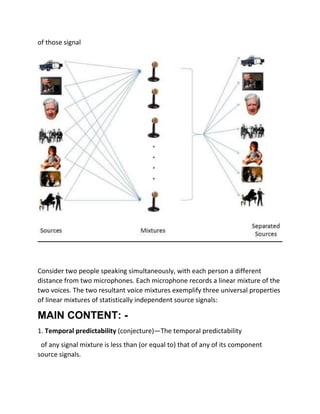
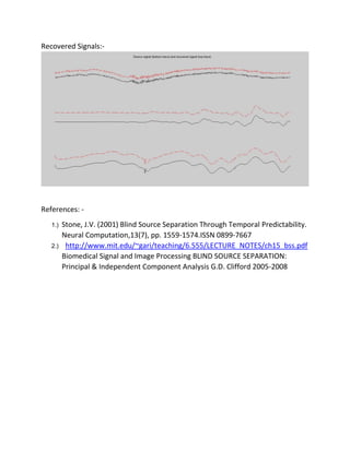
INDIAN INSTITUTE OF TECHNOLOGY ROORKEE
Blind Source Separation
Kamal Bhagat (14115056)
ABSTRACT: -
Blind source separation, also known as blind signal separation, is the separation
of a set of source signals from a set of mixed signals, without the aid of
information (or with very little information) about the source signals or the mixing
process. The application of Blind source separation is in several areas like radio
communication, speech and audio applications and biomedical application. In our
project we have taken the three mixtures of three independent audio source
signals and try to recover these source audio signals and we have achieved the
accuracy up to 99.97%.
Acknowledgement –
This proposal describes the research and development that was done to
accomplish the project. The project was carried out under Electronics Section,
Indian Institute of Technology, Roorkee.
First of all, we would like to thank our staff advisor, Mr. Kamal Singh Gotyan for
his guidance and support. His knowledge and ideas have given us a lot of
inspiration. Secondly, we would like to thank our mentors, Padmanabh Pande for
his support, Rahul Ratan Mirdha for giving us information about the
matlabplatform.
Big thanks to all of our friends who helped and supported us directly or indirectly
with the project. Their help and support motivated us to finalize this project.
Introduction: -
Almost every signal measured within a physical system is actually a mixture of
statistically independent source signals. However, because source signals are
usually generated by the motion of mass (e.g., a membrane), the form of
physically possible source signals is underwritten by the laws that govern how
masses can move over time. This suggests that the most parsimonious
explanation for the complexity of a given observed signal is that it consists of a
mixture of simple source signals, each from a different physical source. Here, this
observation has been used as a basis for recovering source signals from mixtures
of those signal
Consider two people speaking simultaneously, with each person a different
distance from two microphones. Each microphone records a linear mixture of the
two voices. The two resultant voice mixtures exemplify three universal properties
of linear mixtures of statistically independent source signals:
MAIN CONTENT: -
1. Temporal predictability (conjecture)—The temporal predictability
of any signal mixture is less than (or equal to) that of any of its component
source signals.
2. Gaussian probability density function—The central limit theorem ensures that
the extent to which the probability density function (pdf) of any mixture
approximates a Gaussian distribution is greater than (or equal to) any of its
component source signals.
3. Statistical Independence—The degree of statistical independence between any
two signal mixtures is less than (or equal to) the degree of independence between
any two source signals.
Problem Definition and Temporal Predictability. Consider a set of K statistically
independent source signals s ={ s1 | s2 | ··· | sK}t, where the ith row in s is a signal
si measured at n time points (the superscript t denotes the transpose operator). It
is assumed throughout this article that source signals are statistically
independent, unless stated otherwise. A set of M ≥ K linear mixtures x ={ x1 | x2 |
··· | xM}t of signals in s can be formed with an M×K mixing matrix A: x = As. If the
rows of A are linearly independent,3 then any source signal si can be recovered
from x with a 1 × M matrix Wi: si = Wix. The problem to be addressed here
consists in finding an unmixing matrix W ={W1 | W2 |···|WK}t such that each row.
Measuring Signal Predictability. The definition of signal predictability F used here
is:
F(Wi,x) = logV(Wi,x) U(Wi,x)
= logVi Ui
= log Pn τ=1(yτ − yτ)2 Pn τ=1(˜ yτ − yτ)2
, (1.1)
where yτ = Wixτ is the value of the signal y at time τ, and xτ is a vector of K signal
mixture values at time τ. The term Ui reflects the extent to which yτ is predicted
by a short-term moving average ˜ yτ of values in y. In contrast, the term Vi is a
measure of the overall variability in y, as measured by the extent to which yτ is
predicted by a long-term moving average yτ of values in y. The predicted values ˜
yτ and yτ of yτ are both exponentially weighted sums of signal values measured
up to time (τ − 1), such that recent values have a larger weighting than those in
the distant past:
˜ yτ = λS ˜ y(τ−1) + (1 − λS) y(τ−1) :0 ≤ λS ≤ 1 yτ = λL y(τ−1) + (1 − λL) y(τ−1) :0 ≤ λL ≤
1. (1.2)
The half-life hL of λL is much longer (typically 100 times longer) than the
corresponding half-life hS of λS. The relation between a half-life h and the
parameter λ is defined as λ = 2−1/h. Note that maximizing only Vi would result in
a high variance signal with no constraints on its temporal structure. In contrast,
minimizing only
Blind Source Separation Using Temporal Predictability U would result in a DC
signal. In both cases, trivial solutions would be obtained for Wi because Vi can be
maximized by setting the norm of Wi to be large, and U can be minimized by
setting Wi = 0. In contrast, the ratio Vi/Ui can be maximized only if two
constraints are both satisfied: (1) y has a nonzero range (i.e., high variance) and
(2) the values in y change slowly over time. Note also that the value of F is
independent of the norm of Wi, so that only changes in the direction of Wi affect
the value of F4.
A Physical Interpretation. The solutions found by the method are the
eigenvectors(W1,W2,...,WM)of the matrix( ˜ C−1C).These eigenvectors are
orthogonal in the metrics C and ˜ C:
Results:-
Three experiments using the method described above were implemented in
Matlab. In each experiment, K source signals were used to generate M.
Table1: Correlation Magnitudes Between Source Signals and Signals Recovered
from Mixtures of Source Signals with Different pdfs.
Source Signals
s1 s2 s3
y1 0.000 0.001 1.000
y2 1.000 0.000 0.000
y3 0.042 0.999 0.002
K signal mixtures, using a K × K mixing matrix, and these M mixtures were used as
input to the method. Each mixture signal was normalized to have zero-mean and
unit variance. Each mixing matrix was obtained using the Matlab randn function.
The short-term and long-term half-lives defined in equation (1.2) were set to hS =
1 and hL = 9000, respectively. Correlations between source signals and recovered
signals are reported as absolute values. Results were obtained in under 60
seconds on a Macintosh G3(233MHz) for all experiments reported here, using non
optimized Matlab code. In each case, an un-mixing matrix was obtained as the
solution to a generalized eigenvalue problem using
the Matlab eigenvalue function W = eig(C, ˜ C)
Signal Mixtures: -
Recovered Signals:-
References: -
1.) Stone, J.V. (2001) Blind Source Separation Through Temporal Predictability.
Neural Computation,13(7), pp. 1559-1574.ISSN 0899-7667
2.) http://www.mit.edu/~gari/teaching/6.555/LECTURE_NOTES/ch15_bss.pdf
Biomedical Signal and Image Processing BLIND SOURCE SEPARATION:
Principal & Independent Component Analysis G.D. Clifford 2005-2008

Project_report_BSS

  • 1.
    INDIAN INSTITUTE OFTECHNOLOGY ROORKEE Blind Source Separation Kamal Bhagat (14115056)
  • 2.
    ABSTRACT: - Blind sourceseparation, also known as blind signal separation, is the separation of a set of source signals from a set of mixed signals, without the aid of information (or with very little information) about the source signals or the mixing process. The application of Blind source separation is in several areas like radio communication, speech and audio applications and biomedical application. In our project we have taken the three mixtures of three independent audio source signals and try to recover these source audio signals and we have achieved the accuracy up to 99.97%.
  • 3.
    Acknowledgement – This proposaldescribes the research and development that was done to accomplish the project. The project was carried out under Electronics Section, Indian Institute of Technology, Roorkee. First of all, we would like to thank our staff advisor, Mr. Kamal Singh Gotyan for his guidance and support. His knowledge and ideas have given us a lot of inspiration. Secondly, we would like to thank our mentors, Padmanabh Pande for his support, Rahul Ratan Mirdha for giving us information about the matlabplatform. Big thanks to all of our friends who helped and supported us directly or indirectly with the project. Their help and support motivated us to finalize this project.
  • 4.
    Introduction: - Almost everysignal measured within a physical system is actually a mixture of statistically independent source signals. However, because source signals are usually generated by the motion of mass (e.g., a membrane), the form of physically possible source signals is underwritten by the laws that govern how masses can move over time. This suggests that the most parsimonious explanation for the complexity of a given observed signal is that it consists of a mixture of simple source signals, each from a different physical source. Here, this observation has been used as a basis for recovering source signals from mixtures
  • 5.
    of those signal Considertwo people speaking simultaneously, with each person a different distance from two microphones. Each microphone records a linear mixture of the two voices. The two resultant voice mixtures exemplify three universal properties of linear mixtures of statistically independent source signals: MAIN CONTENT: - 1. Temporal predictability (conjecture)—The temporal predictability of any signal mixture is less than (or equal to) that of any of its component source signals.
  • 6.
    2. Gaussian probabilitydensity function—The central limit theorem ensures that the extent to which the probability density function (pdf) of any mixture approximates a Gaussian distribution is greater than (or equal to) any of its component source signals. 3. Statistical Independence—The degree of statistical independence between any two signal mixtures is less than (or equal to) the degree of independence between any two source signals. Problem Definition and Temporal Predictability. Consider a set of K statistically independent source signals s ={ s1 | s2 | ··· | sK}t, where the ith row in s is a signal si measured at n time points (the superscript t denotes the transpose operator). It is assumed throughout this article that source signals are statistically independent, unless stated otherwise. A set of M ≥ K linear mixtures x ={ x1 | x2 | ··· | xM}t of signals in s can be formed with an M×K mixing matrix A: x = As. If the rows of A are linearly independent,3 then any source signal si can be recovered from x with a 1 × M matrix Wi: si = Wix. The problem to be addressed here consists in finding an unmixing matrix W ={W1 | W2 |···|WK}t such that each row. Measuring Signal Predictability. The definition of signal predictability F used here is: F(Wi,x) = logV(Wi,x) U(Wi,x) = logVi Ui = log Pn τ=1(yτ − yτ)2 Pn τ=1(˜ yτ − yτ)2 , (1.1) where yτ = Wixτ is the value of the signal y at time τ, and xτ is a vector of K signal mixture values at time τ. The term Ui reflects the extent to which yτ is predicted by a short-term moving average ˜ yτ of values in y. In contrast, the term Vi is a measure of the overall variability in y, as measured by the extent to which yτ is predicted by a long-term moving average yτ of values in y. The predicted values ˜ yτ and yτ of yτ are both exponentially weighted sums of signal values measured up to time (τ − 1), such that recent values have a larger weighting than those in the distant past:
  • 7.
    ˜ yτ =λS ˜ y(τ−1) + (1 − λS) y(τ−1) :0 ≤ λS ≤ 1 yτ = λL y(τ−1) + (1 − λL) y(τ−1) :0 ≤ λL ≤ 1. (1.2) The half-life hL of λL is much longer (typically 100 times longer) than the corresponding half-life hS of λS. The relation between a half-life h and the parameter λ is defined as λ = 2−1/h. Note that maximizing only Vi would result in a high variance signal with no constraints on its temporal structure. In contrast, minimizing only Blind Source Separation Using Temporal Predictability U would result in a DC signal. In both cases, trivial solutions would be obtained for Wi because Vi can be maximized by setting the norm of Wi to be large, and U can be minimized by setting Wi = 0. In contrast, the ratio Vi/Ui can be maximized only if two constraints are both satisfied: (1) y has a nonzero range (i.e., high variance) and (2) the values in y change slowly over time. Note also that the value of F is independent of the norm of Wi, so that only changes in the direction of Wi affect the value of F4. A Physical Interpretation. The solutions found by the method are the eigenvectors(W1,W2,...,WM)of the matrix( ˜ C−1C).These eigenvectors are orthogonal in the metrics C and ˜ C: Results:- Three experiments using the method described above were implemented in Matlab. In each experiment, K source signals were used to generate M. Table1: Correlation Magnitudes Between Source Signals and Signals Recovered from Mixtures of Source Signals with Different pdfs. Source Signals s1 s2 s3
  • 8.
    y1 0.000 0.0011.000 y2 1.000 0.000 0.000 y3 0.042 0.999 0.002 K signal mixtures, using a K × K mixing matrix, and these M mixtures were used as input to the method. Each mixture signal was normalized to have zero-mean and unit variance. Each mixing matrix was obtained using the Matlab randn function. The short-term and long-term half-lives defined in equation (1.2) were set to hS = 1 and hL = 9000, respectively. Correlations between source signals and recovered signals are reported as absolute values. Results were obtained in under 60 seconds on a Macintosh G3(233MHz) for all experiments reported here, using non optimized Matlab code. In each case, an un-mixing matrix was obtained as the solution to a generalized eigenvalue problem using the Matlab eigenvalue function W = eig(C, ˜ C) Signal Mixtures: -
  • 9.
    Recovered Signals:- References: - 1.)Stone, J.V. (2001) Blind Source Separation Through Temporal Predictability. Neural Computation,13(7), pp. 1559-1574.ISSN 0899-7667 2.) http://www.mit.edu/~gari/teaching/6.555/LECTURE_NOTES/ch15_bss.pdf Biomedical Signal and Image Processing BLIND SOURCE SEPARATION: Principal & Independent Component Analysis G.D. Clifford 2005-2008