Audio processing is an area where signal separation is considered as a fascinating works, potentially offering a vivid range of new scope and experience in professional and personal context. The objective of Blind Audio Source Separation is to separate audio signals from multiple independent sources in an unknown mixing environment. This paper addresses the key challenges in BASS and unsupervised approaches to counter these challenges. Comparative performance analysis of Fast-ICA algorithm and Convex Divergence ICA for Blind Source Separation is presented with the help of experimental result. Result reflects Convex Divergence ICA with α=-1 gives more accurate estimate in comparison of Fast ICA..

1. Int. Journal of Electrical & Electronics Engg. Vol. 2, Spl. Issue 1 (2015) e-ISSN: 1694-2310 | p-ISSN: 1694-2426
29 NITTTR, Chandigarh EDIT-2015
Blind Audio Source Separation (Bass): An
Unsuperwised Approach
Naveen Dubey1
, Rajesh Mehra2
1
ME Scholar, Dept. Of Electronics, NITTTR, Chandigarh, India
2
Associate Professor, Dept. Of Electronics, NITTTR, Chandigarh, India
1
naveen_elex@rediffmail.com
ABSTRACT: Audio processing is an area where signal
separation is considered as a fascinating works, potentially
offering a vivid range of new scope and experience in
professional and personal context. The objective of Blind
Audio Source Separation is to separate audio signals from
multiple independent sources in an unknown mixing
environment. This paper addresses the key challenges in
BASS and unsupervised approaches to counter these
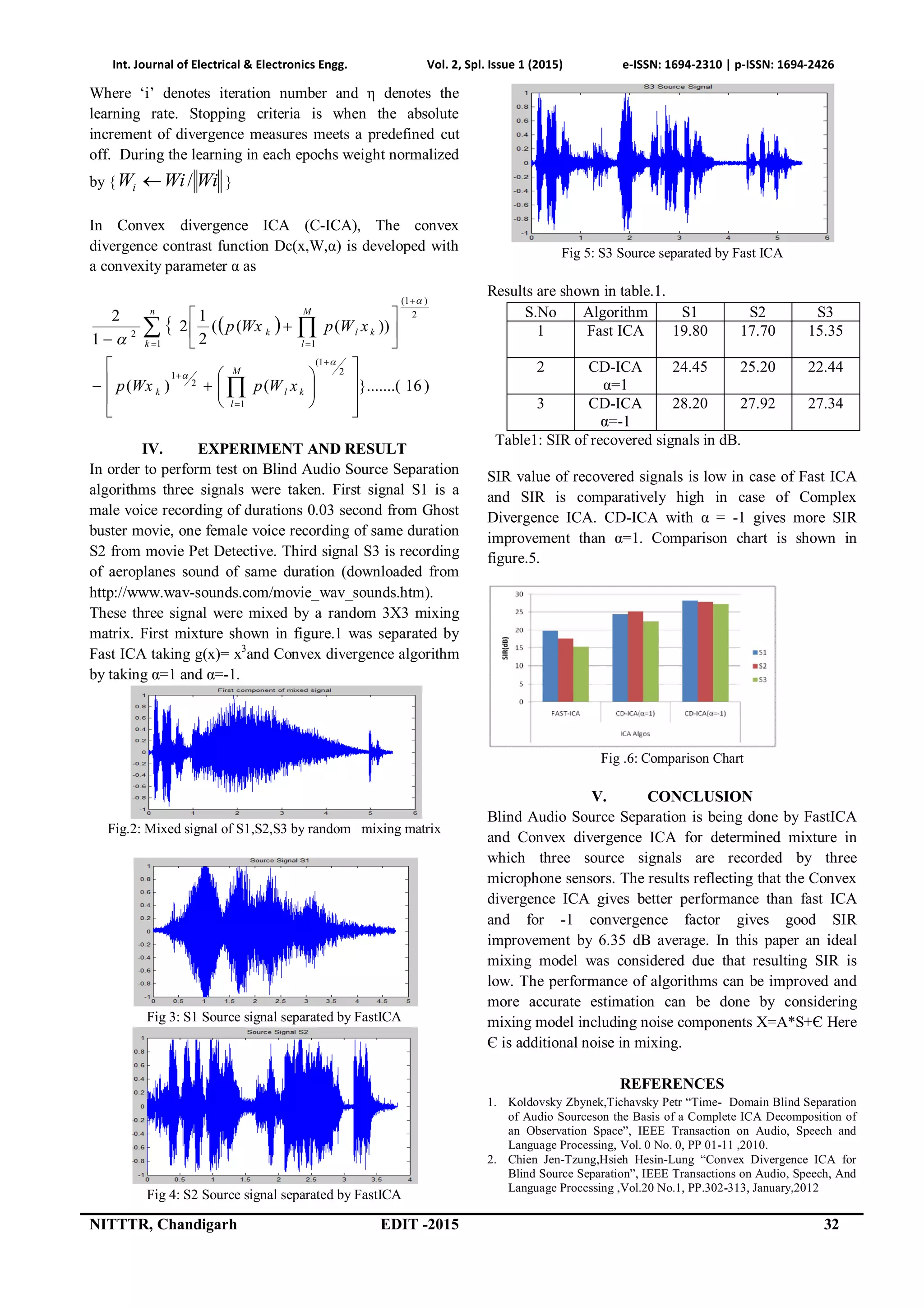
challenges. Comparative performance analysis of Fast-ICA
algorithm and Convex Divergence ICA for Blind Source
Separation is presented with the help of experimental result.
Result reflects Convex Divergence ICA with α=-1 gives more
accurate estimate in comparison of Fast ICA . In this paper
algorithms are considered for ideal mixing situation where no
noise component taken in to account.
Index Terms: BASS, ICA, Fast-ICA, SIR, Convex Divergence,
Entropy, Unsupervised Learning.
I. INTRODUCTION
Blind separation of at a time active audio sources is very
interesting area for researchers and is a popular task in
field of audio signal processing motivated by many
emerging applications , like distant-talking speech
communication, human-machine applications, in
intelligence for national security in call interception, hand-
free and so on[1].
The key objective of BASS is to retrieve ‘p’ audio source
from a convolutive mixture of audio signals captured by
‘m’ microphone sensors, can be mathematically
represented as.
  )1(,.....,1,)()(
0
1
0
miknskhnx
p
j
Mij
k
jiji   


Where:
Xi(n) : ‘m’ recorded audio (observed) signals
Sj(n) : ‘p’ original (audio) signals.
The original signals Sj(n) are unknown in “blind” scenario.
In actual sense, the mixing system is a multi-input multi-
output (MIMO) linear filter with source microphone
impulse response hij, each of length Mij,[2].
The BASS system can be understood by another
mathematical model of matrix convolution [3]. As the
model for mixing
X(t) = A(t) ʘ S(t) (2)
Fig.1 BASS System Diagram
And the model for un-mixing using BASS
)()(ˆ tWtS  ʘ X(t) (3)
Where:
 ʘ denotes matrix convolution
 t is the sample index
 S(t)= [S1(t). . . . .Sp(t)]T is the vector of ‘p’
sources.
 X(t)= [X1(t). . . . Xm(t)]T is observed signal from
‘m’ microphones.
 )(ˆ tS =[ )(1ˆ tS . . . . )(ˆ tpS ]T is the output of
reconstructed sources.
 A(t) is the M X P X L mixing array,
 W(t) is the P X M X L un mixing array,
A(t) and W(t) can also be considered as M X P and P X M
matrices, where each element is an FIR filter of length L,
[4].
Previously discussed model is a an ideal representation of
BASS model where number of audio sources is equal to
number of microphone sensors, termed as complete model
or critically determined model. The modelling can be more
complex for more practicability of application, as if
number of microphone sensors more than number of audio
source (m > p), termed as overdetermined or over complete
model. If number of sources are greater than number of
microphone sensors (p > m) , named as underdertermined
or under complete model [5,6]. Inclusion of noise
component and delay between microphones, echo makes
BASS problem more complex.ICA is a dominant
algorithm for blind source separation problem and based
on metrics of likelihood function, negentropy, kurtosis and

2. Int. Journal of Electrical & Electronics Engg. Vol. 2, Spl. Issue 1 (2015) e-ISSN: 1694-2310 | p-ISSN: 1694-2426
NITTTR, Chandigarh EDIT -2015 30
minimum mutual information (MMI). The remaining
content of this paper is organized as follows. Section II
reviews of ICA algorithm. Section III reviews Fast-ICA
and Convex Divergence ICA for BASS. Section IV
summarizes the experiment on simulation and real data.
Conclusion drawn on the basis of experimental results in
Section V.
II. INDEPENDENT COMPONENT ANALYSIS
A big challenge in statistics and concerned areas is to pick
a suitable representation of multivariate data. Here
representation stands for data transformation such that its
essential, hidden structure is made more transparent or
accessible. Blind Audio source separation considered as a
convolutive mixture, as in equation (2) and to separate out
source component estimate can be generated by equation
(3). W(t) represents unmixing matrix and key objective of
ICA algorithms to find out most accurate value of matrix
W(t). It is analogous to designing of a neural structure to
short out clustering problem and various learning methods
can be adapted for updation of W(t). To implement ICA
for BASS problem certain set of assumption and pre-
processing needed.
A. ASSUMPTIONS AND AMBIGUITIES IN ICA
FRAMEWORK
There are certain assumptions of the signal characteristics
to implement ICA in proper manner as pointed out
The sources being considered are statistically independent.
Suppose there are two random variables x1 and x2. The
random variable x1 is independent of x2, if the information
content of x1 does not provide any information about x2
and vice versa. Here x1 and x2 are random signals
generated from two different physical activities which are
not related to each other.
X1 and x2 are said to be independent if and only if the
expression for joint Probability Density function is:
)2()1()2,1( 212,1 xpxpxxP xx  (4)
The independent component has non-Gaussian
distribution.
This assumption is very essential because it not possible to
separate Gaussian signal using ICA framework. The sum
of non- Gaussian signal signals is itself a Gaussian and it is
the principle reason behind non separability of Gaussian
signals. Kurtosis and entropy are the techniques to ensure
non-Gaussianity of signals, described in next subsection.
The mixing matrix is invertible
This assumption have very clear mathematical support that
if mixing matrix is not invertible, then unmixing matrix we
seek to estimate cam not even exist.
ICA suffers from two inherent ambiguities; these are (i)
permutation ambiguity and (ii) magnitude and scaling
ambiguity. In ICA the order of the estimated independent
components are not specified and due that the permutation
ambiguity is inherent in BSS. This ambiguity is to be
expected, so we do not impose any restriction on order and
all permutations are equally valid. Magnitude and scaling
ambiguity comes into the picture because true variance of
the independent components cannot be estimated.
Fortunately in most applications this ambiguity is not
significant and to avoid this assumption can be made that
each sources has unit variance [6].
B. NON- GAUSSIANITY
As per central limit theorem the nature of a sum of
independent signals with arbitrary distribution tends
towards a Gaussian distribution under specific conditions.
So Gaussian signal can be assumed as linear combinations
of number of independent signals. The separation of
independent signal can be achieved by making the linear
signal transform as non-Gaussian as it could be. To ensure
non-Gaussianity there are certain commonly used
measures.
i. Kurtosis
In probability theory kurtosis is a measure of
“peakedness”. When data is preconditions to have unit
variance, kurtosis of signal (x) can be calculated by fourth
moment of data.
244
}){(3}{)( xExExkurt  (5)
Here E{.}- Expectation
Now if signal assumed having zero mean and ‘x’ has been
normalized such that its variance is equal to one E{x2}=1.
.3}{)( 4
 xExkurt (6)
Gaussian nature of distribution can measured on the basis
of kurtosis by following criteria’s
If:
Kurt(x) = 0 : x is Gaussian
Kurt(x)>0 : x is super-Gaussian/ platy kurtotic
Kurt(x)< 0:x is sub-Gaussian /lepto kutotic
Kurtosis is a computationally simple process, as it has a
linearity property. But kurtosis is sensitive to outlier data
and its statistical significance is poor. Kurtosis is not
enough robust for ICA.
ii. Entropy
According to information theory, entropy termed as
average amount of information contained in each message
received. The minimum amount of mutual information
ensures better separation along with non-Gaussianity.
Uniformity of signal corresponds to maximum entropy and
entropy is considered as randomness of a signal. Entropy
for a continuous valued signal (x), called the differential
entropy, and is defined as

3. Int. Journal of Electrical & Electronics Engg. Vol. 2, Spl. Issue 1 (2015) e-ISSN: 1694-2310 | p-ISSN: 1694-2426
31 NITTTR, Chandigarh EDIT-2015
 dxxpxpxH )(log)()( (7)
Highest value of entropy represents the Gaussian signal
and low value of entropy shows the spiky nature of signal.
In ICA estimated non-Gaussianity must be ensured, which
is zero for Gaussian signal and non zero for non-Gaussian
signal. Hence entropy minimization is a prime concern in
ICA estimation. A normalized version of entropy gives a
new measure for non-Gaussianity termed as Negentropy J
which is defined as,
)()()( xHXgaussHxJ  (8)
For Gaussian signal negentropy is zero and non-
Gaussianity achieved by negentropy maximization.
C. ICA PREPROCESSING
Before implementing ICA algorithms certain pre-
processing steps are carried out.
i. Centering
It is a commonly performed pre-processing step to centre
the observation vector X by subtracting its mean vector
m=E{x}. The centered observation vector can be presented
as follows
mxXc  (9)
The mixing matrix remains same after this pre-processing,
so unmixing matrix can be estimated by centered data after
then actual estimated can be derived.
ii. Whitening
Whitening the observation vector X is a very useful
practice. Whitening involves linearly transforming the
observation vector such that its components are
uncorrelated and have unit variance [4].The whitening
vector satisfies the following relationship
..}{ IxxE T
ww 
(10)
A simple approach to perform the whitening
transformation is to apply eigenvalue decomposition
(EVD)[]of x.
TT
VDVxxE }{ (11)
Here: }( T
xxE : co variance matrix of x
V: eigenvector of }( T
xxE
D:diagonal matrix of eigenvalues
Whitening is very simple and efficient process that
significantly reduces the computational complexity of ICA.
III. ICA ALGORITHMS
A. FAST ICA
Fast ICA is a fixed point algorithm that applies statistics
for the recovery of independent source components. Fast
ICA uses a simple estimate of Negentropy based on
negentropy maximization that requires the use of
appropriate non-linearities for unsupervised learning rules
of neural networks [10].
Fixed point algorithms are based on the mutual
information minimization. This can be written as
dx
xif
xf
xfxI
xi
x
x

)(
)(
log)()(
(12)
Minimization of mutual information leads to ICA solution.
For MI minimization negentropy needs to minimized
[7].For the estimation of negentropy, the pdf estimation of
the random vector variable required and it is hard to obtain
by calculation. Hyvarinen [8] proposed a method to
calculate negentropy. Let ‘x’ be a whitened random
variable. Then the approximation of J(x) is given by
2
)})({)}({()( uGExGExJ  (13)
Where G(.) is a nonquadratic function and g(.) is first
derivative G(.), u is a Gaussian variable with unit variance
and zero mean. Nonlinear parameter for convergence is
g(.) should grow slowly as given[2].
)tanh()(
)(
2
3
1
xxg
xxg


(14)
Iteration for unmixing matrix given as
#Choose an initial weight matrix W+
For i=1:1++: C
While W+ changes
 
WxS
WWWOutput
W
W
W
WWWWW
WxWg
M
xWxg
M
W
T
c
i
i
i
k
i
k
k
T
iii
i
T
i
TT
ii















ˆ
:
)('
1
)(
1
1
1
1
B. CONVEX DIVERGENCE
Convex divergence is a learning algorithm through
minimizing a divergence measure D(x,W) given a
unmixing matrix W and a set of M- dimensional input
observations x={x1,. . . . . . . ,xn}. Data is pre-processed
by centering and whitening . The unmixing matrix can be
estimated by the gradient descent method [9].
.
)(
))(,(
)()1(
iW
iWxD
iWiW


 
(15)

4. Int. Journal of Electrical & Electronics Engg. Vol. 2, Spl. Issue 1 (2015) e-ISSN: 1694-2310 | p-ISSN: 1694-2426
NITTTR, Chandigarh EDIT -2015 32
Where ‘i’ denotes iteration number and η denotes the
learning rate. Stopping criteria is when the absolute
increment of divergence measures meets a predefined cut
off. During the learning in each epochs weight normalized
by { WiWiWi / }
In Convex divergence ICA (C-ICA), The convex
divergence contrast function Dc(x,W,α) is developed with
a convexity parameter α as
  
)16}.......(()(
))(((
2
1
2
1
2
2
1(
1
2
1
2
)1(
1 1
2



























 

 




M
l
klk
n
k
M
l
klk
xWpWxp
xWpWxp
IV. EXPERIMENT AND RESULT
In order to perform test on Blind Audio Source Separation
algorithms three signals were taken. First signal S1 is a
male voice recording of durations 0.03 second from Ghost
buster movie, one female voice recording of same duration
S2 from movie Pet Detective. Third signal S3 is recording
of aeroplanes sound of same duration (downloaded from
http://www.wav-sounds.com/movie_wav_sounds.htm).
These three signal were mixed by a random 3X3 mixing
matrix. First mixture shown in figure.1 was separated by
Fast ICA taking g(x)= x3
and Convex divergence algorithm
by taking α=1 and α=-1.
Fig.2: Mixed signal of S1,S2,S3 by random mixing matrix
Fig 3: S1 Source signal separated by FastICA
Fig 4: S2 Source signal separated by FastICA
Fig 5: S3 Source separated by Fast ICA
Results are shown in table.1.
S.No Algorithm S1 S2 S3
1 Fast ICA 19.80 17.70 15.35
2 CD-ICA
α=1
24.45 25.20 22.44
3 CD-ICA
α=-1
28.20 27.92 27.34
Table1: SIR of recovered signals in dB.
SIR value of recovered signals is low in case of Fast ICA
and SIR is comparatively high in case of Complex
Divergence ICA. CD-ICA with α = -1 gives more SIR
improvement than α=1. Comparison chart is shown in
figure.5.
Fig .6: Comparison Chart
V. CONCLUSION
Blind Audio Source Separation is being done by FastICA
and Convex divergence ICA for determined mixture in
which three source signals are recorded by three
microphone sensors. The results reflecting that the Convex
divergence ICA gives better performance than fast ICA
and for -1 convergence factor gives good SIR
improvement by 6.35 dB average. In this paper an ideal
mixing model was considered due that resulting SIR is
low. The performance of algorithms can be improved and
more accurate estimation can be done by considering
mixing model including noise components X=A*S+Є Here
Є is additional noise in mixing.
REFERENCES
1. Koldovsky Zbynek,Tichavsky Petr “Time- Domain Blind Separation
of Audio Sourceson the Basis of a Complete ICA Decomposition of
an Observation Space”, IEEE Transaction on Audio, Speech and
Language Processing, Vol. 0 No. 0, PP 01-11 ,2010.
2. Chien Jen-Tzung,Hsieh Hesin-Lung “Convex Divergence ICA for
Blind Source Separation”, IEEE Transactions on Audio, Speech, And
Language Processing ,Vol.20 No.1, PP.302-313, January,2012

5. Int. Journal of Electrical & Electronics Engg. Vol. 2, Spl. Issue 1 (2015) e-ISSN: 1694-2310 | p-ISSN: 1694-2426
33 NITTTR, Chandigarh EDIT-2015
3. Fu Gen-Shen et al. “Complex Indpendent Component Analysis Using
Three Type of Diversity: Non-Gaussianity, Nonwhiteness, and
Noncircularity” IEEE Transactions on Signal Processing, Vol 63,
No.3,PP.794-805 Feb 2015
4. Vincent Emmanuel, Bertin Nancy, G. Remi, Bimbot Frederic “From
Blind to Guided Audio Source Separation”, IEEE Signal Processing
Magazine,PP. 107-115, May,2014
5. Naik R. Ganesh, Kumar K Dinesh “An Overview of Independent
Component Analysis and Its Applications”, Iformatica 35, PP.63-
81,2011
6. Emmanuel Vincent, Rémi Gribonval, and Cédric Févotte,”
Performance Measurement in Blind Audio Source Separation” IEEE
Transactions on Audio, Speech, and Language processing, vol. 14,
no. 4,PP 1462-1469,July 2006
11. C.D. Meyer, Matrix Analysis and Applied linear Algebra, Cambridge,
UK,2000.
10. Zhiming Li and Genke Yang, “Blind separationof Mixed Audio
Signals Based on Improved Fast ICA”, CISP, pp.1638-1642, 2013
9. S. Amari, “Natural gradient efficiency in learning” Neural
Computing, vol.10, pp.251-276, 1998
Analysis”.John Wiley& Sons, New York,2001.
Science, vol.4707, pp.431-444, 2007.
8. A. Hyvarine, J. Karhuenen and E. Oja, “Independent Component
7. S.L. Lin and P.C Tung “Application of modified ICA to secure
communication in chaotic systems” Lecture Notes in Computer