The document summarizes the trust region algorithm for solving unconstrained optimization problems. It begins by introducing trust region methods and comparing them to line search algorithms. The basic trust region algorithm is then outlined, which approximates the objective function within a region using a quadratic model at each iteration. It discusses solving the trust region subproblem to find a step that minimizes the model within the trust region. Finally, it introduces the Cauchy point and double dogleg step as methods for solving the subproblem.

1. The Trust Region
Algorithm
Two Semester Project
Abstract: Trust region methods are modern techniques for solving
optimization problems. In this paper the operations and underlying theory
of the trust-region algorithms is investigated. The convergence properties
of the basic algorithm in relation to the Cauchy point are also examined.
The basic algorithm is then extended by incorporating Powell’s double dog-
leg step. The final algorithm is programmed in MATLAB and implemented
on a test problem. The performance of the algorithm is then compared with
the Newton-Raphson method.
2012
ChristianAdom(k0849957)
KingstonUniversity
4/27/2012

2. 2
Contents Page
Introduction.......................................................................................................................................3
The Trust Region Method....................................................................................................................6
[2] (B.T.R.A) Basic Trust Region Algorithm............................................................................................8
The trust region sub-problem..............................................................................................................9
Local Model Minimiser....................................................................................................................9
The Cauchy point and the Model Decrease.....................................................................................10
Convergence of the algorithm....................................................................................................11
Cases 1: Model minimiser within Trust region.............................................................................11
Case1b: Model Minimiser outside Trust region ...........................................................................12
Case 2: Negative Curvature........................................................................................................13
Powell’s Double Dog-leg step.........................................................................................................13
Dogleg Parameters....................................................................................................................14
The Double-Dog leg Algorithm...................................................................................................15
MATLAB Implementation..................................................................................................................16
Code for Newton’s Method...........................................................................................................16
Code For Trust Region Double Dog Leg...........................................................................................19
Test Problem....................................................................................................................................28
Analysis on Test problem ..................................................................................................................34
Conclusion .......................................................................................................................................35
References.......................................................................................................................................35

3. 3
Introduction
Line search algorithms are one of two basic methods for solving optimization problems. These
algorithms employ descent directions as a search direction, with the aim of reducing some
objective function by taking an appropriate step length within this search direction.[1]
Examples of such methods are: The steepest (gradient) Descent, Newton and Quasi Newton
Methods.[1]
In this paper an alternative method of solving unconstrained optimization problems will be
examined, namely the Trust region method.
Trust region methods have been developed for over five decades and are commonly founded in
the field of non-linear parameter estimation.[2]
The development of the method is primarily attributed to three individuals who seem to have
developed it independently;
 Kenneth Levenberg (1944) – Researched adding a multiple of the identity to the Hessian
as a stabilization/damping procedure in an attempt to derive the solution of a number
of nonlinear least-square problem.[2]
 Morrison (1960) - In his a paper on trajectory tracking Morrison developed on
Levenberg’s ideas, in which convergence of the estimation algorithm is enhanced by
minimizing a quadratic model. In Morison’s paper a technique based on eigen-value
decomposition is given to compute the model’s minimum within a chosen sphere.[2]
 Donald Marquardt (1963) – While researching the link between damping the Hessian
and reducing the length of the step Marquardt came to a similar conclusion as Morrison
by proving that minimizing a damped model is similar to minimizing the original model
within a restricted region.[2]
The trust region method is based primarily on the idea of approximating some objective
function within a certain region at each iteration.
In contrast to line search algorithms (which also employ this idea of solving approximate
models) the approximate model used with the trust region algorithm is constrained within a
region at the current iterate with the idea that the model can only be “trusted” within this
bound. This is the main difference between the trust region and line search algorithms.
The most the most prevalent of line search algorithms are the Newton and Quasi-Newton
methods, which widely used within the field of optimization due to their fast (quadratic)
convergence properties, given that certain conditions are satisfied.

4. 4
The trust region algorithm is in fact a modification of such methods, in that it restricts the
Newton step within the bounds of the trust region.[3]
This approach might at first seem counter-intuitive as an important feature of any algorithm is
to reach the optimal point as quickly as possible.
However the trust region approach addresses (and remedies) the major drawbacks inherent in
Newton’s method and is put in place to safe-guard Newton’s method from diverging. In fact
most modern algorithms use a combination of line search and trust region methods for
unconstrained optimization problems.
As a reminder we know that Newton’s method will converge to a local minima if:
1. Start point is not too far from the optimal point (less negative curvature to deal with)
2. The Hessian matrix (or its approximation) is positive definite at each iteration.
In fact the requirement for a positive definite matrix is to ensure that the curvature of the
function is always positive.
Now it can be proven that global convergence can still be achieved given an indefinite Hessian if
a constraint of the form:‖ 𝑠 𝑘‖2 ≤ ∆ 𝑘is imposed on the stepsize. [4]
This idea of constraining the step-size is one of the distinct features of the trust region method,
where ∆ 𝑘is defined as the “trust region radius at iteration k” the region where we trust the
model/approximation of the objective function to be “a faithful representation” of the
objective function.
Consider the case where in a search for a minimum we encounter a region of negative
curvature (Hessian negative definite), in this case Newton’s method will most likely diverge
whilst the trust region algorithm is designed to calculate a step length of ‖ 𝑠 𝑘‖2 = ∆ 𝑘 which will
Usually be a long step in the direction of the minimum[4]. We will explore this idea in more
detail at a later stage.
The major drawback to the trust region method is that in order to obtain in the step 𝑠 𝑘 a
minimization problem subject to one constraint (known as the Trust region sub-problem) must
be solved. This is not trivial and can be both computationally expensive time consuming,
especially if a there are a large number of variables.
Finally it is worth noting that trust region methods have a wide range of applications within the
fields of science, engineering and even the social sciences. The table below gives a few some
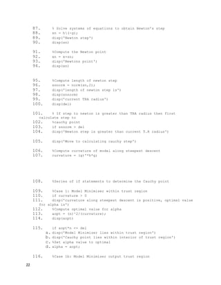
examples of some of its applications

5. 5
Table of Application [2]
AppliedMathematics Min-cost flows,Bi-level programming, Least-
distance problems, Boundary values problems,
Partial and ordinary differential equations
Physics Fluid dynamics, optics, electromagnetism
Chemistry PhysicalChemistry, Chemical engineering,
Molecular modelling, Mass transfer
Engineering Transportation analysis, Radar applications,
Circuit design
Economics&sociology – Game theory, Random utility models,
Financial portfolio management

6. 6
The Trust Region Method
Given an unconstrained optimization problem of the form:
min 𝑓( 𝑥) |𝑥𝜖ℝ [1.0]
where: f(x) is assumed to be a real valued, twice continuously differentiable.
The trust region is defined as:
𝐵 𝑘 = { 𝑥𝜖ℝ 𝑛
|‖ 𝑥 − 𝑥 𝑘‖2 ≤ Δ 𝑘} [1.1] [5]
where: Δ 𝑘 is the trust region radius at the kth iteration
Now, it is worth noting that shape of the trust region can differ depending on the type of norm
used (as shown in Figure [1.0]), and some authors have suggested that the shape of the trust
region should be adjusted with each iteration, however for simplicity this paper will only
consider the 2-norm.
Fig[1.0] – Showing various shapes of the trust region.
The trust-region approach to solving [1.0] is by first approximating the objective function by a
model function, this is because the model function will usually be easier to handle and less
costly to evaluate.

7. 7
This model function is usually chosen to be quadratic, and is based on the idea that a function
can be expanded locally by its Taylor series:
𝑓( 𝑥 + 𝛿𝑥) = 𝑓( 𝑥) + 𝛿𝑥𝑓′( 𝑥) +
𝛿𝑥
2
𝑓′′( 𝑥)+ ⋯ [1.2]
Now [1.2] can be extended from one dimension to many dimensions so that the quadratic
model can be defined as:
𝑚 𝑘( 𝑥 𝑘 + 𝑠) = 𝑓( 𝑥 𝑘)+ 𝑔 𝑘
𝑇
𝑠 𝑘 +
1
2
𝑠 𝑘
𝑇
𝐻 𝑘 𝑠 𝑘 [1.3] [6]
where: g is the gradient vector (or its approximation) and [2]H is the Hessian matrix (the square
matrix of second order partial derivatives of a function) and s is the trial step.
Note: In real life problems (where there a large number variables) the Hessian matrix is usually
approximated by methods such DFP and BFGS. However in this paper the analytical Hessian will
be used since the test problems will only consist of a small number of (at most three) variables.
Once the model function is constructed the algorithm is then concerned with finding a step that
sufficiently reduces the model within the trust region. This step is what we call the trial step.
Two further conditions are also placed on this step:
𝑥 𝑘 + 𝑠 𝑘 𝜖 𝐵 𝑘 𝑎𝑛𝑑 ‖ 𝑠 𝑘‖2 ≤ Δ 𝑘 [1.4]
Once a step that satisfies the conditions mentioned above is obtained the algorithm needs a
way of deciding whether the reduction predicted by the model using this trial step is in
agreement with the actual reduction observed in the objective function, thus it moves to
evaluate what is known as the ratio of agreement:
( 𝐴𝑐𝑡𝑢𝑎𝑙 𝑅𝑒𝑑𝑢𝑐𝑡𝑖𝑜𝑛)
(𝑃𝑟𝑒𝑑𝑖𝑐𝑡𝑒𝑑 𝑅𝑒𝑑𝑢𝑐𝑡𝑖𝑜𝑛 )
≝ 𝜌 𝑘 =
𝑓( 𝑥 𝑘)−𝑓( 𝑥 𝑘+𝑠 𝑘)
𝑓( 𝑥 𝑘)−𝑚( 𝑥 𝑘+𝑠 𝑘)
[1.5] [7]
If the value obtained from [1.5] shows “adequate” agreement between the reduction in the
model and objective function the trial step is accepted and is used to compute the next iterate.
In addition if this agreement is very close the trust region radius can be expanded with the
hopes that the model function will continue to approximate the objective function well within
an enlarged region.
Alternatively, if the value obtained from [1.5] shows “inadequate” agreement between the
reduction in the model and objective function the trial step is rejected and the trust region
radius is reduced with the hopes that the model function will be better able to approximate the
objective function within a smaller region.

8. 8
(B.T.R.A) Basic Trust Region Algorithm [8]
 Step0: Initialization
o Setk = 0
o Choose an initial guess/searchpoint,define as 𝑥0
o Choose aninitial trustregionradius,define as Δ0
o Choose parameters for 𝜂1, 𝜂2, 𝛾1, 𝛾2 such that:
0 < 𝜂1 ≤ 𝜂2 < 1 𝑎𝑛𝑑 0 < 𝛾1 ≤ 𝛾2 < 1
 Step1: Model Definition
o Define: 𝑚 𝑘( 𝑥 𝑘 + 𝑠) = 𝑓( 𝑥 𝑘)+ 𝑔 𝑇 𝑠 𝑘 +
1
2
𝑠 𝑇 𝐻 𝑘 𝑠 𝑘
 Step2: StepCalculation
o Determine astep 𝑠 𝑘 that reducesthe model subjectto:
 𝑥 𝑘 + 𝑠 𝑘 𝜖 𝐵 𝑘 𝑎𝑛𝑑 ‖ 𝑠 𝑘‖2 ≤ Δ 𝑘
 Step3: Acceptance of trial point:
o Compute: 𝑝 𝑘 =
𝑓( 𝑥 𝑘)−𝑓( 𝑥 𝑘+𝑠 𝑘)
𝑓( 𝑥 𝑘)−𝑚( 𝑥 𝑘+𝑠 𝑘)
 if 𝜌 𝑘 ≥ 𝜂1 Then: 𝑥 𝑘+1 = 𝑥 𝑘 + 𝑠 𝑘
 else if 𝜌 𝑘 < 𝜂1 Then: 𝑥 𝑘+1 = 𝑥 𝑘
 Step4: Trust regionradiusupdate
o Δ 𝑘+1 = {
[Δ 𝑘,∞) 𝑖𝑓: 𝜌 𝑘 ≥ 𝜂2
[ 𝛾1Δ 𝑘,𝛾2Δ 𝑘] 𝑖𝑓: 𝜌 𝑘 𝜖 [𝜂1, 𝜂2]
[ 𝛾1Δ 𝑘, 𝛾2Δ 𝑘] 𝑖𝑓: 𝜌 𝑘 < 𝜂1
 Step5: Stoppingcriteria:
o ‖ 𝑔 𝑘‖2 < 𝜀 𝑎𝑛𝑑 ‖ 𝑠 𝑘‖2 < 𝜀
 Incrementkby 1 and go to step1

9. 9
The trust region sub-problem
An important part of the trust region algorithm is the determination of the trial step 𝑠 𝑘 that
reduces the model defined in [1.3]
In order to obtain this trial step a constrained minimization problem must be solved, this
problem is known as the trust region sub-problem and takes the form:
min 𝑚 𝑘( 𝑠) = 𝑔 𝑇 𝑠 +
1
2
𝑠 𝑇 𝐻𝑠 [1.5] [9]
𝑠𝑢𝑏𝑗𝑒𝑐𝑡 𝑡𝑜: ‖ 𝑠‖2 ≤ Δk
Due to the importance of [1.5] the rest of this paper will be dedicated to examining a small
subset of the known methods for efficiently solving this problem. There are three primary
methods for solving [1.5] namely; The Local Model Minimiser, The Cauchy point and the Double
Dog-Leg step. This paper will be dedicated to examining the last two methods; The Cauchy
point and the Double Dog-Leg step, whilst the Local model minimiser will only be discussed
briefly
Local Model Minimiser
The idea behind this method is to find a step 𝑠 𝑘 which minimizes the model defined in [1.3]
whilst satisfying the constraints, the main advantage of this method is that it usually gives an
asymptotically fast-rate of convergence. It takes the form:
Given:
min 𝑚 𝑘( 𝑠) = 𝑔 𝑇 𝑠 +
1
2
𝑠 𝑇 𝐻𝑠 [1.5] [10]
𝑠𝑢𝑏𝑗𝑒𝑐𝑡 𝑡𝑜: ‖ 𝑠‖2 ≤ Δk
Determine the global minimiser of [1.5] such that:
( 𝐻 + 𝜆𝐼 ) 𝑠 = −𝑔 [1.6] [10]
where: 𝐻 + 𝜆𝐼 ispositive semi-definite
and: lagrangian multiplier 𝜆 ≥ 0
In order to solve [1.5]-[1.6] a unique 𝜆∗
must be found which satisfies the condition above. This
is usually done by applying Newton’s method [10].
If a unique 𝜆∗
can found at each iteration then a step 𝑠 𝑘 that sufficiently reduces the model can
be computed and consequently global convergence can be achieved. Yet this method has some
major drawbacks, of all the methods available it is the most computational expensive, since

10. 10
obtaining the solution to [1.5]-[1.6] will require the factorisation of 𝐻 + 𝜆𝐼 and matrix
factorization can be very demanding [11].
Therefore rather than obtaining the actual local model minimiser at each iteration, algorithms
have been designed that rather seek to approximate it. A few examples include preconditioned
conjugate Gradient, Leven-Marquardt and Powell’s Dog-Leg method [12].
The Cauchy point and the Model Decrease
Before discussing the double dog leg method, it important to examine what is known as the
Cauchy point.
As discussed above, all trust region algorithms seek to minimise some model or approximation
of some objective function within a specific region. A simple way to do this is examine the
behaviour of the model along the steepest descent direction, as this is where can expect a
significant reduction in the model.
The minimum of a model is found along the Cauchy arc, the point where we can expect the
greatest decrease in the model is known as the Cauchy point and the step taken towards such a
point is called the Cauchy step.
𝑩 𝒌
𝒔 𝑪
−𝛁𝒇(𝒙)
𝒙 𝒄

11. 11
[6]The Cauchy point is defined mathematically as:
𝑥 𝑘
𝐶
≝ 𝑥 + 𝑠 𝑘
𝐶
[1.7]
Where:
𝑠 𝑘
𝐶
= −𝛼 𝑘 𝑔 𝑘 is the Cauchy step [1.71]
And:
𝛼 ≥ 0
𝑥 𝑘
𝐶
𝜖 𝐵 𝑘
Convergenceofthealgorithm
It can be proved that the achievable model decrease at each iteration is given by:
𝑃𝑟𝑒𝑑𝑖𝑐𝑡𝑒𝑑 𝑅𝑒𝑑𝑢𝑐𝑡𝑖𝑜𝑛 ≝ 𝑓( 𝑥 𝑘)− 𝑚 𝑘( 𝑥 𝑘 + 𝑠 𝑘) ≥
1
2
‖ 𝑔 𝑘‖2 min [∆,
‖ 𝑔 𝑘‖2
1 + ‖ 𝐻 𝑘‖2
] [1.8] [13]
This proof will not be shown in this paper however some of the important convergence
properties of the algorithm will be explored.
To determine the Cauchy point there are three particular cases to consider. These cases are
discussed below.
Cases1: Model minimiser withinTrustregion
Let:
𝑚 𝑘( 𝑥 𝑘 − 𝛼𝑔 𝑘) ≝ 𝑚( 𝑥 𝑘
𝐶) [1.9]
Then applying [1.3] we can write [1.9] as:
𝑚( 𝑥 𝑘
𝐶) = 𝑓𝑘( 𝑥 𝑘)− 𝛼‖ 𝑔 𝑘‖2
2
+
1
2
𝛼2
𝑔 𝑘
𝑇
𝐻 𝑘 𝑔 𝑘 [2.0] [14]
Now introduce the condition:
𝑔 𝑘
𝑇
𝐻 𝑘 𝑔 𝑘 > 0 [2.1]
(i.e. - Require that the curvature of the model along the descent direction to be positive)
This is to ensure convergence to a local minimum. Now, if the above condition holds then the
optimal value of alpha (denoted 𝛼∗
) which minimises the model (defined in [2.0]) along the
Cauchy arc is found by the usual method of differentiation and equating to zero.
Thus:
Figure [1.1] - contour plot of the Rosenbrock function
An example of the Cauchy point within the trust region
The red dot represents the Cauchy point
The dashed arrow represents the Cauchy arc in the negative descent direction
The Cauchy step is the distance from the current search point 𝑥 𝑐 to the Cauchy point and is
denoted is here by 𝑠 𝐶

12. 12
𝜕 (𝑚 𝑘( 𝑥 𝑘
𝐶))
𝜕𝛼
= −‖ 𝑔 𝑘‖2
2
+ 𝛼 𝑘 𝑔 𝑘
𝑇
𝐻 𝑘 𝑔 𝑘 [2.2]
Then equating [2.2] to zero and solving for alpha gives:
𝛼 𝑘
∗
=
‖ 𝑔 𝑘‖2
2
𝑔 𝑘
𝑇
𝐻 𝑘 𝑔 𝑘
[2.3]
Now we know from [1.71] that the Cauchy step is given by: 𝑠 𝑘
𝐶
= −𝛼 𝑘 𝑔 𝑘 thus we can expect
the Cauchy point to lie within the trust region when:
𝛼∗
𝑘‖ 𝑔 𝑘‖2 ≤ ∆ 𝑘 [2.4]
If this is the case then it is expedient to choose the value for alpha as the optimal value defined
by [2.3].
Therefore we have: 𝛼 𝑘 = 𝛼 𝑘
∗
[2.5]
Now replacing [2.3] into [2.0] will allow us to deduce the amount of decrease we can expect to
achieve from the model when the Cauchy point is within the trust region.
Thus:
𝑚( 𝑥 𝑘
𝐶) = 𝑓𝑘( 𝑥 𝑘)− (
‖ 𝑔 𝑘‖2
2
𝑔 𝑘
𝑇
𝐻 𝑘 𝑔 𝑘
) ‖ 𝑔 𝑘‖2
2
+
1
2
(
‖ 𝑔 𝑘‖2
2
𝑔 𝑘
𝑇
𝐻 𝑘 𝑔 𝑘
)
2
𝑔 𝑘
𝑇
⇒ 𝑓𝑘( 𝑥 𝑘) − 𝑚 𝑘( 𝑥 𝑘
𝐶) =
1
2
(
‖ 𝑔 𝑘‖2
4
𝑔 𝑘
𝑇
𝐻 𝑘 𝑔 𝑘
) [2.6]
Case1b:Model MinimiseroutsideTrustregion
This is a sub-case of Case 1 rather than a separate case on it’s own as we assume that condition
[2.1] still holds.
If the model minimiser lies outside the trust region:
𝛼 𝑘‖ 𝑔 𝑘‖2 > ∆ 𝑘 [2.7] [14]
Then it is prudent to take a step back towards the boundary of the trust region to avoid
divergence.
Thus the appropriate value in this case for the parameter alpha is given by:
𝛼 𝑘‖ 𝑔 𝑘‖2 = Δ 𝑘
⇒ 𝛼 𝑘 =
Δ 𝑘
‖ 𝑔 𝑘‖2
[2.8]
Now replacing [2.8] into [2.0] will allow us to deduce the amount of decrease we can expect to
achieve from the model when the Cauchy point is outside the trust region.
Thus:
𝑚( 𝑥 𝑘
𝐶) = 𝑓𝑘( 𝑥 𝑘)− (
Δ 𝑘
‖ 𝑔 𝑘‖2
) ‖ 𝑔 𝑘‖2
2
+
1
2
(
Δ 𝑘
‖ 𝑔 𝑘‖2
)
2
𝑔 𝑘
𝑇
𝐻 𝑘 𝑔 𝑘
⇒ 𝑓𝑘( 𝑥 𝑘)− 𝑚 𝑘( 𝑥 𝑘
𝐶) = ‖ 𝑔 𝑘‖2 Δ 𝑘 −
1
2
(
Δ 𝑘
‖ 𝑔 𝑘‖2
)
2
𝑔 𝑘
𝑇
𝐻 𝑘 𝑔 𝑘 [2.9]

13. 13
Case2: NegativeCurvature
This case corresponds to the situation when [2.1] is violated, giving:
𝑔 𝑘
𝑇
𝐻 𝑘 𝑔 𝑘 < 0 [3.0]
Then [3.0] implies that:
𝑚( 𝑥 𝑘
𝐶) = 𝑓𝑘( 𝑥 𝑘)− 𝛼 𝑘‖ 𝑔 𝑘‖2
2
+
1
2
𝛼2
𝑔 𝑘
𝑇
𝐻 𝑘 𝑔 𝑘 ≤ 𝑓𝑘( 𝑥 𝑘)− 𝛼 𝑘‖ 𝑔 𝑘‖2
2 [3.1] [14]
(Since the highlighted term will be negative due to [3.0])
Now since the Cauchy point is on the boundary of the trust region we replace [2.8] into [3.1] to
obtain:
𝑚( 𝑥 𝑘
𝐶) = 𝑓𝑘( 𝑥 𝑘)− Δ 𝑘‖ 𝑔 𝑘‖2 +
1
2
(
Δ 𝑘
‖ 𝑔 𝑘‖2
)
2
𝑔 𝑘
𝑇
𝐻 𝑘 𝑔 𝑘 ≤ 𝑓𝑘( 𝑥 𝑘) − (
Δ 𝑘
‖ 𝑔 𝑘 ‖2
) ‖ 𝑔 𝑘‖2
2 [3.2]
(Since the highlighted term will be negative due to [3.0])
⇒ 𝑚( 𝑥 𝑘
𝐶) − 𝑓𝑘( 𝑥 𝑘) ≤ 𝑓𝑘( 𝑥 𝑘)− (
Δ 𝑘
‖ 𝑔 𝑘‖2
)‖ 𝑔 𝑘‖2
2
as the amount of decrease we can expect to achieve from the model when we have negative
curvature.
This concludes the analysis on the Cauchy point.
Powell’s DoubleDog-leg step
As discussed above the Cauchy step provides a trial point which gives a model decrease, it
greatest advantage is that it computationally cheap to obtain. However this method is based on
steepest descent direction thus continues steps towards this Cauchy point will probably result in
a slow converging method for certain methods. This is perhaps the reason why it is very rarely
used as the sole search method.
This bring us to the Double Dog leg step attributed to Powell this method is works in a similar
way to the Levenburg-Marquardt method in that it uses combinations of the steepest descent
and Guass-Newton direction. It addresses the slow convergence the steepest descent and the
difficulties of computing the exact local Model minimiser.
The algorithm begins by computing the step to the Newton point (See page 15). If this point is
within the trust region radius the Newton step is taken as the trial step and the sub-problem is
solved, thus we proceed to step 3 of the Basic Trust region algorithm (defined on page 4).
If the Newton point is outside the trust region radius, then the algorithm first computes the
step to the Cauchy point. If this point is on the boundary of the trust region radius then no
better step can be achieved thus Cauchy step is taken as the trial step and the sub-problem is
solved, thus we proceed to step 3 of the Basic Trust region algorithm (defined on page 4)
If the Cauchy point is within the trust region the algorithm connects a line from the Cauchy
point to a point in the Gauss-Newton direction, such that the dogleg step is found this along the
line. In fact the main purpose of the algorithm is to calculate an exact step of ‖ 𝑠‖2 = Δ 𝑘 (i.e a
step to the boundary of the trust region) where we can expect a good model reduction.

14. 14
The double dogleg step has two important properties that make the process of finding the step
mathematical sound and computationally efficient. Firstly as the algorithm moves from the
current iterate to the Cauchy point, all the way to the new point, the distance from the current
iterate increases monotonically. Meaning for any ∆ 𝑘≤ ‖ 𝐻𝑐
−1
∇𝑓( 𝑥 𝑐)‖2 there is a unique point
𝑥 𝑘+1 on the dogleg curve (see figure 1.2) such that ‖ 𝑠 𝑘‖2 = ∆ 𝑘. Secondly the value of the
quadratic model defined in [1.3] will decrease monotonically as 𝑠 𝑘 moves along the current
iterate, to the Cauchy point all the way to the new point [15].
Fig[1.2] – Showsthe processof computingthe doglegstep
Dogleg Parameters
So far the general form of the algorithm has been given, now the mathematics behind it is to be
examined. The mathematical parameters for calculating the double dogleg were developed in
1979 by Dennis and Mei:
The Newton step is given by:
𝑠 𝑁
= −𝐻−1
𝑔 [3.3]
Note: In practice the inverse Hessian is not computed, rather a systemof non-linear equations
are solved.
The step in the Newton direction is given by:
[9] 𝑠 𝑁̂
= 𝜂𝑠 𝑁 [3.4] [16]
where:
[9] 𝜂 = 0.8𝛾 + 0.2 𝑓𝑜𝑟 𝛾 ≤ 𝜂 ≤ 1 [3.5] [16]
𝑩 𝒌
𝒙 𝒄
−𝛁𝒇(𝒙)
𝒙 𝑪
𝑵̂
𝑺 𝑵

15. 15
This is a scaling factor used to reduce the length of the Newton step.
and:
[9] 𝛾 =
‖ 𝑔 𝑘‖2
4
( 𝑔 𝑇 𝐻𝑔)(𝑔 𝑇 𝐻−1 𝑔)
[3.6] [16]
Now given these initial set of parameters the dogleg step is given by:
[9] 𝑠 𝐷
= 𝑠 𝐶
+ 𝜆(𝑠 𝑁̂
− 𝑠 𝐶
) [3.7] [16]
where:
0 ≤ 𝜆 ≤ 1 𝑎𝑛𝑑 𝑠 𝐶
𝑖𝑠 𝑑𝑒𝑓𝑖𝑛𝑒𝑑 𝑏𝑦 [1.71]
Now the aim of the algorithm is to take a step that sufficiently reduces the model at each
iteration, a possible means of achieving this aimis to take a step to boundary of the trust
region, i.e our step must satisfy:
‖ 𝑠 𝑘
𝐷‖ = Δ 𝑘 [3.8]
This brings us to a second issue, the algorithm must find a value of 𝜆 that satisfies [3.8], this
value is found by solving the quadratic equation:
‖𝑠 𝐶
+ 𝜆(𝑠 𝑁̂
− 𝑠 𝐶
)‖
2
2
= Δ2
[3.9]
Then [3.9] can be expanded and re-written as:
‖𝑠 𝑁̂
− 𝑠 𝐶
‖
2
2
𝜆2
+ 2((𝑠 𝑁̂
− 𝑠 𝐶
)
𝑇
𝑠 𝐶
)𝜆 + ‖ 𝑠 𝐶 ‖2
2
− Δ2
= 0 [4.0]
Then applying the quadratic formula:
−𝑏± √𝑏2
−4𝑎𝑐
2𝑎
to [4.0] gives:
𝜆 =
−2 ((𝑠 𝑁̂
− 𝑠 𝐶
)
𝑇
𝑠 𝐶
)± √2 ((𝑠 𝑁̂
− 𝑠 𝐶 )
𝑇
𝑠 𝐶 )
2
− 4(‖𝑠 𝑁̂
− 𝑠 𝐶 ‖
2
2
)(‖ 𝑠 𝐶‖2
2
− Δ2)
2(‖𝑠 𝑁̂
− 𝑠 𝐶 ‖2
2
)
[4.1]
Note: the algorithm always chooses the positive root of [4.1] since we must have 0 ≤ 𝜆 ≤ 1
TheDouble-DoglegAlgorithm
 Step1:
o Compute 𝑠 𝑁 [3.3]
 If 𝑠 𝑁is lessthanTrust regionradiusgotto step 3 of B.T.R.A (Pg4)
 Else if 𝑠 𝑁isgreaterthan Trust regionradiusproceedtostep2
 Step2:
o Compute: 𝑠 𝐶 [1.71]
 If 𝑠 𝐶is equal tothan Trust regionradiusgotto step 3 of B.T.R.A (Pg4)
 Else if 𝑠 𝑁islessthan Trust regionradiusproceedtostep3
 Step3:
o Compute: 𝑠 𝐷 [3.7]
o Got to step 3 of B.T.R.A (Pg4)

16. 16
MATLAB Implementation
In this section of the report we put the theory into practice by implementing the trust region
algorithm in a computer program. The main purpose of the programs is not only to test the
convergence properties of the trust region algorithm but also to compare it with the Newton-
Raphson Method.
All the computer programs have been written using Matlab software.
Code for Newton’s Method
The Newton-Raphson method was simple to code, the main work of the algorithm is done in
line 73 where it solves a systemof non-linear equations.
1. %MATLAB CODE
2. %______________________________________________________________________
_
3. %______________________________________________________________________
_
4. %Newton Algorithm
5. disp('****')
6. disp('Welcome Newton Method)
7. disp('By: Christian Adom, Kingston University, k0849957')
8. disp('****')
9. %Display Objective function to minimize
10. disp('Minimize the function:f = -10*x(1)^2 + 10*x(2)^2+
4*sin(x(1)*x(2))-2*x(1)+x(1)^4')
11. %Display 3D plot of function
12. ezmeshc('-10*x^2 + 10*y^2+ 4*sin(x*y)-2*x+x^4',[-2,2,-2,2])
13. disp('****')
14. %Local Minimum of function
15. xo = [2.3029;-0.3409];
16. disp('known minimum of function at')
17. disp(xo)
18. %Ask the user to supply a start point for search
19. in1 = input('Please Enter starting x value:');
20. in2 = input ('Please Enter starting y value:');
21. %Store user input into a vector
22. x = [in1;in2];
23. disp('****')
24. disp('Start point')
25. disp(x)

17. 17
26. %Stopping criteria
27. normtol = input('Stop search when either 2-norm of gradient or
step length is less than?:');
28. disp('****')
29. %Ask user to specify maximum number iterations allowed
30. Maxit = input('Please enter maximum number of iterations
allowed:');
31. disp('****')
32. %Initiate a while loop will terminate when either the 2-norm of
the gradient or step length is less than the specified tolerance value
or the maximum number of iterations are exceeded
33. while (n > normtol && iteration < Maxit)
34. iteration = iteration +1;
35. disp('**********************************')
36. disp('iteration')
37. disp(iteration)
38. disp('***********************************')
39. %Compute value of Objective function current point
40. f = -10*x(1)^2 + 10*x(2)^2+ 4*sin(x(1)*x(2))-2*x(1)+x(1)^4;
41. disp('Current Objective function Value')
42. disp(f)
43. % Compute Gradient vector of objective function at current point
44. g = [-20*x(1)+4*cos(x(1)*x(2))*x(2)-
2+4*x(1)^3;20*x(2)+4*cos(x(1)*x(2))*x(1)];
45. disp('Current Gradient vector value')
46. disp(g)
47. %Compute Hessian Matrix of objective function at current point
48. h = [-20-4*sin(x(1)*x(2))*x(2)^2+12*x(1)^2,-
4*sin(x(1)*x(2))*x(1)*x(2)+4*cos(x(1)*x(2));-
4*sin(x(1)*x(2))*x(1)*x(2)+4*cos(x(1)*x(2)),20-
4*sin(x(1)*x(2))*x(1)^2];
49. disp('Current Hessian Matrix Value')
50. disp(h)
51. %Extract First element in Hessian matrix
52. FirstElement = h(1,1);
53. %Compute Determinant of Hessian Matrix

18. 18
54. dm = det(h);
55. disp('The determinant is')
56. disp(dm)
57. %Evaluate A series of if statements to determine the nature of
the Hessian
58. if FirstElement > 0 && dm > 0
59. disp('Hessian is positive definite')
60. elseif FirstElement < 0 && dm > 0
a. disp('Hessian is negative definite')
61. elseif FirstElement >= 0 && dm >=0
62. disp('Hessian is positive semidefinite')
63. elseif FirstElement <= 0 && dm >= 0
64. disp('Hessian is negative semidefinite')
65. else
66. disp('Hessian is indefinite')
67. end
68. %Compute 2-Norm of gradient
69. n = norm(g,2);
70. disp('2 norm of gradient')
71. disp(n)
72. %Solve systems of equations to obtain Newton’s step
73. sn = h(-g);
74. disp('Newton step')
75. disp(sn)
76. %Compute the Newton point
77. xn = x+sn;
78. disp('Newtons point')
79. disp(xn)
80. %Store new value in x
81. x = xn;
82. end
83. disp('***********************************************************
**********')
84. disp('RESULTS')
85. disp('***********************************************************
**********')
86. disp('Distance from current point to optimal solution')
87. %disp(distSol)
88. disp('The 2 norm of gradient is')
89. disp(n)
90. disp('The 2 norm of step length is')

19. 19
91. disp(TrialStepNorm)
92. disp('Location of minimum at')
93. disp(x)
94. disp('Function value at minimum')
95. disp(f)
96. disp('Total Number of iterations')
97. disp(iteration)
98. %Display a contour plot of objective function
99. fplot4=@(x,y) -10*x.^2 + 10*y.^2+ 4*sin(x*y)-2*x+x.^4;
100. ezcontour(fplot4,[-5,5,-5,5],49)
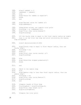
Code For Trust Region Double Dog Leg
The code for the double dog leg is large and complex, it totals approximately 300 lines of code,
this due to the fact that it incorporates three methods (Steepest Descent, Newton & Dogleg) to
solve the trust region sub-problem.
1. %MATLAB CODE
2. %______________________________________________________________________
_
3. %______________________________________________________________________
_
4. %Basic Trust region Algorithm
5. %The Double Dogleg Step
6. disp('****')
7. disp('Welcome to the Trust region Algorithm')
8. disp('Double Dogleg Step')
9. disp('By: Christian Adom, Kingston University, k0849957')
10. disp('****')
11. %Display objective function to minimize
12. disp('Minimize the function:f = -10*x(1)^2 + 10*x(2)^2+
4*sin(x(1)*x(2))-2*x(1)+x(1)^4')
13. Display a 3D plot of function
14. ezmeshc('-10*x^2 + 10*y^2+ 4*sin(x*y)-2*x+x^4',[-2,2,-2,2])
15. disp('****')
16. %Local minimum of objective function
17. xo = [2.3029;-0.3409];
18. disp('known minimum of function at')
19. disp(xo)
20. %Ask the user to supply a start point for search
21. in1 = input('Please Enter starting x value:');

20. 20
22. in2 = input ('Please Enter starting y value:');
23. %Store values as a vector
24. x = [in1;in2];
25. disp('****')
26. disp('Start point')
27. disp(x)
28. %Trust region radius modification values
29. eta1 = 0.01;
30. eta2 = 0.9;
31. %Iteration counter
32. iteration = 0;
33. %Dummy value for norms
34. n = 10;
35. TrialStepNorm = 10;
36. %Stopping criteria
37. normtol = input('Stop search when either 2-norm of gradient or
step length is less than?:');
38. disp('****')
39. %Ask user to specify maximum number iterations allowed
40. Maxit = input('Please enter maximum number of iterations
allowed:');
41. %Maxit = M1;
42. disp('****')
43. %Ask user to supply an initial Trust region radius
44. del = input('Please enter intial trust region radius:');
45. disp('intial trust region radius')
46. disp(del)
47. %Initiate a while loop will terminate when either the 2-norm of
the gradient or step length is less than the specified tolerance value
or the maximum number of iterations are exceeded
48. while (n > normtol && iteration < Maxit)
49. iteration = iteration +1;
50. disp('**********************************')
51. disp('iteration')
52. disp(iteration)
53. disp('***********************************')
54. %Compute value of Objective function at current point

21. 21
55. f = -10*x(1)^2 + 10*x(2)^2+ 4*sin(x(1)*x(2))-2*x(1)+x(1)^4;
56. disp('Current Objective function Value')
57. disp(f)
58. % Compute Gradient vector of objective function at current point
59. g = [-20*x(1)+4*cos(x(1)*x(2))*x(2)-
2+4*x(1)^3;20*x(2)+4*cos(x(1)*x(2))*x(1)];
60. disp('Current Gradient vector value')
61. disp(g)
62. %Compute Hessian Matrix of objective function at current point
63. h = [-20-4*sin(x(1)*x(2))*x(2)^2+12*x(1)^2,-
4*sin(x(1)*x(2))*x(1)*x(2)+4*cos(x(1)*x(2));-
4*sin(x(1)*x(2))*x(1)*x(2)+4*cos(x(1)*x(2)),20-
4*sin(x(1)*x(2))*x(1)^2];
64. disp('Current Hessian Matrix Value')
65. disp(h)
66. %Extract first element in Hessian matrix
67. FirstElement = h(1,1);
68. %Compute Determinant of Hessian Matrix
69. dm = det(h);
70. disp('The determinant is')
71. disp(dm)
72. %Evaluate a series of if statements to determine the nature of
the Hessian
73. if FirstElement > 0 && dm > 0
74. disp('Hessian is positive definite')
75. elseif FirstElement < 0 && dm > 0
a. disp('Hessian is negative definite')
76. elseif FirstElement >= 0 && dm >=0
77. disp('Hessian is positive semidefinite')
78. elseif FirstElement <= 0 && dm >= 0
79. disp('Hessian is negative semidefinite')
80. else
81. disp('Hessian is indefinite')
82. end
83. %Compute 2-Norm of gradient
84. n = norm(g,2);
85. disp('2 norm of gradient')
86. disp(n)

22. 22
87. % Solve systems of equations to obtain Newton’s step
88. sn = h(-g);
89. disp('Newton step')
90. disp(sn)
91. %Compute the Newton point
92. xn = x+sn;
93. disp('Newtons point')
94. disp(xn)
95. %Compute length of newton step
96. snnorm = norm(sn,2);
97. disp('length of newton step is')
98. disp(snnorm)
99. disp('current TRA radius')
100. disp(del)
101. % If step to newton is greater than TRA radius then first
calculate step to
102. %cauchy point
103. if snnorm > del
104. disp('Newton step is greater than current T.R radius')
105. disp('Move to calculating cauchy step')
106. %Compute curvature of model along steepest descent
107. curvature = (g)'*h*g;
108. %Series of if statements to determine the Cauchy point
109. %Case 1: Model Minimiser within trust region
110. if curvature > 0
111. disp('curvature along steepest descent is positive, optimal value
for alpha is')
112. %Compute optimal value for alpha
113. aopt = (n)^2/(curvature);
114. disp(aopt)
115. if aopt*n <= del
a. disp('Model Minimizer lies within trust region')
b. disp('Cauchy point lies within interior of trust region')
c. %Set alpha value to optimal
d. alpha = aopt;
116. %Case 1b: Model Minimiser output trust region

23. 23
117. else
a. disp('Model Minimiser outside trust region')
b. disp('Compute Cauchy point at boundary of trust region')
118. %Compute a value of alpha that sets Cauchy point at boundary of
trust region
a. alpha = (del)/n;
119. end
120. %Case 2: Negative curvature
121. else
122. disp('curvature along steepest descent is negative')
123. disp('Compute Cauchy point at boundary of trust region')
124. %Compute a value of alpha that sets Cauchy point at boundary of
trust region
125. alpha = (del)/n;
126. end
127. %Compute Cauchy step
128. sc = -alpha*g;
129. disp('cauchy step is')
130. disp(sc)
131. %Compute Cauchy point
132. xc = x + sc;
133. disp('cauchy point is')
134. disp(xc)
135. %Compute length of Cauchy step
136. scnorm = norm(sc,2);
137. disp('length of the cauchy step is:')
138. disp(scnorm);
139. disp('current TRA radius')
140. disp(del)
141. %if length of Cauchy step is less than tra radius then calculate
dogleg step
142. if abs(scnorm-del)> 0.0001
143. %Note: Since matlab doesnt regonize == sign when dealing with
144. %floating point values we use the abs value of
145. %the difference subject to a tolerance to evaluate if the two
values are equal
146. disp('***************')
147. disp('***************')
148. disp('Cauchy step is less than current trust region radius, move
to calculating dogleg step')
149. disp('***************')
150. disp('***************')
151. %Calculation of various parameters needed for Dogleg step (See
report for
152. %explanation)

24. 24
153. gamma = ((n)^4)/((curvature)*(g)'*(-sn));
154. disp('Value for gamma')
155. disp(gamma);
156. kappa = (0.8*gamma) + 0.2;
157. if kappa >= gamma && kappa <= 1
158. disp('value for kappa')
159. disp(kappa);
160. else
161. disp('kappa value out of bounds')
162. disp(kappa)
163. break
164. end
165. %Compute the step towards guass-newton direction
166. snhat = kappa * sn;
167. disp('Step to nhat')
168. disp(snhat);
169. %Compute the nhat point
170. nhat = x + snhat;
171. disp('nhat point')
172. disp(nhat);
173. %Compute length of snhat step
174. snhatnorm = norm(snhat,2);
175. disp('length nhat step ')
176. disp(snhatnorm);
177. disp('current TRA radius')
178. disp(del)
179. v = snhat - sc;
180. %shatnorm = norm(v,2);
181. %disp(v)
182. %Compute value of lambda that satisfies [3.8],[3.9] (See report)
183. lambda1 = (sqrt(-4*((v(1)^2)+(v(2)^2))*((sc(1)^2)+(sc(2)^2)-
((del)^2))+(((2*sc(1)*v(1))+(2*sc(2)*v(2)))^2))-2*sc(1)*v(1)-
2*sc(2)*v(2))/(2*v(1)^2+2*v(2)^2);
184. lambda2 = -(sqrt(-4*((v(1)^2)+(v(2)^2))*((sc(1)^2)+(sc(2)^2)-
((del)^2))+(((2*sc(1)*v(1))+(2*sc(2)*v(2)))^2))-2*sc(1)*v(1)-
2*sc(2)*v(2))/(2*v(1)^2+2*v(2)^2);
185. %A series of if statements to choose the positive root of the
expression for %lambda
186. if lambda1 >= 0
187. lambdaopt = lambda1;

25. 25
188. elseif lambda2 >= 0
189. lambdaopt = lambda2;
190. else
191. disp('Value for lambda is negative')
192. break
193. end
194. disp('Optimal value for lambda is')
195. disp(lambdaopt);
196. %Subproblem solved, now compute trial point
197. TrialStep = sc +lambdaopt*(v);
198. disp('Trial step (using dogleg)')
199. disp(TrialStep)
200. %If the Cauchy step is equal to the trust region radius we simply
201. %use it as the trial new step and avoid calculating the dogleg
step altogether
202. elseif abs(scnorm-del)<0.0001
203. disp('Cauchy step is equal to Trust Region radius, thus use
Cauchy step')
204. TrialStep = sc;
205. disp('')
206. disp('Trial step (using cauchy) is')
207. disp(TrialStep)
208. else
209. disp('Algorithm stopped prematurely')
210. break
211. end
212. %Back to the newton step
213. else
214. disp('Newton step is less than Trust region radius, thus use
newton step')
215. TrialStep = sn;
216. disp('Trial step (using Newton)')
217. disp(TrialStep)
218. end
219. %Compute length of Trial Step
220. TrialStepNorm = norm(TrialStep,2);
221. disp('Trial step length is:')
222. disp(TrialStepNorm);
223. %Compute the trial point

26. 26
224. TrialPoint = x + TrialStep;
225. disp('New Trial point')
226. disp(TrialPoint);
227. %Compute Quadratic Model at current point
228. m = f + (TrialStep)'*(g)+0.5*(TrialStep)'*h*TrialStep;
229. disp('Quadratic Model value')
230. disp(m)
231. %Compute function value at trial point
232. fn = -10*TrialPoint(1)^2 + 10*TrialPoint(2)^2+
4*sin(TrialPoint(1)*TrialPoint(2))-2*TrialPoint(1)+TrialPoint(1)^4;
233. disp('Function value at Trial point')
234. disp(fn)
235. %Compute reduction predicted by the model
236. Predred = f - m;
237. disp('Predicted reduction value is:')
238. disp(Predred)
239. %Compute actual reduction in objective function
240. Actualred = f - fn;
241. disp('Actual reduction')
242. disp(Actualred)
243. %Compute ratio of agreement
244. r = Actualred/Predred;
245. disp('Ratio of agreement')
246. disp(r)
247. %Acceptance of Trial point and trust region radius adjustments
248. if r >= eta2
249. x = TrialPoint;
250. del = 2*del;%Double trust region radius
251. disp('very succesful iteration')
252. disp('New point')
253. disp(x)
254. disp('New trust region radius')
255. disp(del)
256. %Compute distance from current point to optimal solution
257. distSol = norm((x - xo),2);
258. disp('Distance from current point to optimal solution')
259. disp(distSol)
260. elseif r>= eta1 && r < eta2
261. x = TrialPoint;
262. disp('succesful iteration')
263. disp('New point')

27. 27
264. disp(x)
265. disp('Trust region radius remains the same as:')
266. disp(del)
267. %Distance from current point to optimal solution
268. distSol = norm((x - xo),2);
269. disp('Distance from current point to optimal solution')
270. disp(distSol)
271. else
272. disp('unsucessful iteration')
273. disp('Retain current Point at:')
274. disp(x)
275. disp('reduce trust region radius to:')
276. del = del*0.5;%Half trust region radius
277. disp(del)
278. %Distance from current point to optimal solution
279. distSol = norm((x - xo),2);
280. disp('Distance from current point to optimal solution')
281. disp(distSol)
282. end
283. %proceed = input('Press any number to continue:');
284. end
285. disp('***********************************************************
************************')
286. disp('RESULTS')
287. disp('***********************************************************
************************')
288. disp('Distance from current point to optimal solution')
289. disp(distSol)
290. disp('The 2 norm of gradient is')
291. disp(n)
292. disp('The 2 norm of step length is')
293. disp(TrialStepNorm)
294. disp('Location of minimum at')
295. disp(x)
296. disp('Function value at minimum')
297. disp(f)
298. disp('Total Number of iterations')
299. disp(iteration)
300. disp('Final trust region radius')
301. disp(del)
302. %Display contour plot of objective function
303. fplot4=@(x,y) -10*x.^2 + 10*y.^2+ 4*sin(x*y)-2*x+x.^4;
304. ezcontour(fplot4,[-5,5,-5,5],49)

28. 28
Test Problem
In thissectionwe examineone testproblem, while varyingthe start pointof the search.The aimis to
compare the Trust-region(Dogleg) withNewton’sMethodatdifferentstartpoints.
Considerthe function:
f = -10*x(1)^2 + 10*x(2)^2+ 4*sin(x(1)*x(2))-2*x(1)+x(1)^4

29. 29
This function has two local minimum located at:
𝑥∗
= (2.3, −0.3) 𝑎𝑛𝑑 𝑥∗
= (−2.3,0.3)

30. 30
Search 1 (Newton)
Newton Method
By: Christian Adom, Kingston University, k0849957
****
Minimize the function:f = -10*x(1)^2 + 10*x(2)^2+
4*sin(x(1)*x(2))-2*x(1)+x(1)^4
****
known minimum of function at
2.3029
-0.3409
Please Enter starting x value:2
Please Enter starting y value:-1
****
Start point
2
-1
Stop search when either 2-norm of gradient or step
length is less than?:0.05
****
Please enter maximum number of iterations
allowed:50
*********************************************
RESULTS
*********************************************
Distance from current point to optimal solution
The 2 norm of gradient is
0.0115
The 2 norm of step length is
10
Location of minimum at
2.3066
-0.3323
Function value at minimum
-31.1807
Total Number of iterations
4
Search 1 (Trust Region Dog Leg)
Welcome to the Trust region Algorithm
Double Dogleg Step
By: Christian Adom, Kingston University,k0849957
****
Minimizethe function:f = -10*x(1)^2 + 10*x(2)^2+
4*sin(x(1)*x(2))-2*x(1)+x(1)^4
****
known minimum of function at
2.3029
-0.3409
PleaseEnter startingx value:2
PleaseEnter startingy value:-1
****
Start point
2
-1
Stop search when either 2-norm of gradient or step length is less
than?:0.05
****
Pleaseenter maximum number of iterations allowed:50
****
Pleaseenter initial trustregion radius:1
initial trustregion radius
1
*********************************************
RESULTS
*********************************************
Distancefrom current point to optimal solution
0.0094
The 2 norm of gradient is
0.0088
The 2 norm of step length is
1.9999e-004
Location of minimum at
2.3066
-0.3323
Function value atminimum
-31.1807
Total Number of iterations
6
Final trustregion radius
0.0625

31. 31
Search 2 (Newton)
****
Newton Method
By: Christian Adom, Kingston University, k0849957
****
Minimize the function:f = -10*x(1)^2 + 10*x(2)^2+
4*sin(x(1)*x(2))-2*x(1)+x(1)^4
****
known minimum of function at
2.3029
-0.3409
Please Enter starting x value:3
Please Enter starting y value:-2
****
Start point
3
-2
Stop search when either 2-norm of gradient or step
length is less than?:0.05
****
Please enter maximum number of iterations
allowed:50
*********************************************
RESULTS
*********************************************
Distance from current point to optimal solution
The 2 norm of gradient is
9.0599e+004
The 2 norm of step length is
10
Location of minimum at
-28.1660
-354.4216
Function value at minimum
1.8934e+006
Total Number of iterations
50
Search 2 (Trust RegionDogleg)
Welcome tothe Trust regionAlgorithm
Double DoglegStep
By: ChristianAdom, Kingston University,k0849957
****
Minimize the function:f =-10*x(1)^2 + 10*x(2)^2+
4*sin(x(1)*x(2))-2*x(1)+x(1)^4
****
knownminimumof functionat
2.3029
-0.3409
Please Enterstartingx value:3
Please Enterstartingyvalue:-2
****
Start point
3
-2
Stopsearch wheneither2-normof gradientorsteplengthis
lessthan?:0.05
****
Please entermaximumnumberof iterationsallowed:50
****
Please enterinitial trustregionradius:1
Initial trustregionradius
1
*************************************************
RESULTS
*************************************************
Distance fromcurrentpointto optimal solution
0.0094
The 2 norm of gradientis
0.0188
The 2 norm of steplengthis
4.2610e-004
Locationof minimumat
2.3066
-0.3323
Functionvalue atminimum
-31.1807
Total Numberof iterations
23
Final trustregionradius
1

32. 32
Search 3 (Newton)
Newton Method
By: Christian Adom, Kingston University, k0849957
****
Minimize the function:f = -10*x(1)^2 + 10*x(2)^2+
4*sin(x(1)*x(2))-2*x(1)+x(1)^4
known minimum of function at
2.3029
-0.3409
Please Enter starting x value:5
Please Enter starting y value:4
****
Start point
5
4
Stop search when either 2-norm of gradient or step
length is less than?:0.05
Please enter maximum number of iterations
allowed:50
*********************************************
RESULTS
*********************************************
Distance from current point to optimal solution
The 2 norm of gradient is
1.3979e+003
The 2 norm of step length is
10
Location of minimum at
7.0870
-20.1869
Function value at minimum
7.0395e+003
Total Number of iterations
50
Search 3 (Trust regionDogleg)
****
Welcome tothe Trust regionAlgorithm
Double DoglegStep
By: ChristianAdom, KingstonUniversity,k0849957
****
Minimize the function:f =-10*x(1)^2 + 10*x(2)^2+
4*sin(x(1)*x(2))-2*x(1)+x(1)^4
****
knownminimumof functionat
2.3029
-0.3409
Please Enterstartingx value:5
Please Enterstartingyvalue:4
****
Start point
5
4
Stopsearch wheneither2-normof gradientorsteplengthis
lessthan?:0.05
****
Please entermaximumnumberof iterationsallowed:50
****
Please enterinitial trust regionradius:1
Initial trustregionradius
1
*************************************************
RESULTS
*************************************************
Distance fromcurrentpointto optimal solution
4.5627
The 2 norm of gradientis
0.0124
The 2 norm of steplengthis
3.6198e-004
Locationof minimumat
-2.2102
0.3297
Functionvalue atminimum
-22.1430
Total Numberof iterations
18
Final trustregionradius
0.2500

33. 33
Search 4 (Newton)
****
Newton Method
By: Christian Adom, Kingston University, k0849957
****
Minimize the function:f = -10*x(1)^2 + 10*x(2)^2+
4*sin(x(1)*x(2))-2*x(1)+x(1)^4
****
known minimum of function at
2.3029
-0.3409
Please Enter starting x value:50
Please Enter starting y value:-56
****
Start point
50
-56
Stop search when either 2-norm of gradient or step
length is less than?:0.05
****
Please enter maximum number of iterations
allowed:50
*******************************************
RESULTS
*******************************************
Distance from current point to optimal solution
The 2 norm of gradient is
2.8435e+004
The 2 norm of step length is
10
Location of minimum at
19.2514
-165.7107
Function value at minimum
4.0068e+005
Total Number of iterations
50
Test Problem 4 (Dogleg)
****
Welcome to the Trust region Algorithm
Double Dogleg Step
By: Christian Adom, Kingston University,k0849957
****
Minimizethe function:f = -10*x(1)^2 + 10*x(2)^2+
4*sin(x(1)*x(2))-2*x(1)+x(1)^4
****
known minimum of function at
2.3029
-0.3409
PleaseEnter startingx value:50
PleaseEnter startingy value:-56
****
Start point
50
-56
Stop search when either 2-norm of gradient or step length is
less than?:0.05
****
Pleaseenter maximum number of iterations allowed:50
****
Pleaseenter initial trustregion radius:1
initial trustregion radius
1
****************************************************
RESULTS
****************************************************
Distancefrom current point to optimal solution
0.0094
The 2 norm of gradient is
0.0013
The 2 norm of step length is
2.9134e-005
Location of minimum at
2.3066
-0.3323
Function value atminimum
-31.1807
Total Number of iterations
35
Final trustregion radius
512

34. 34
Analysis on Test problem
This section of the report will attempt to give some analysis on the results produced by the
algorithm Firstly an initial trust region radius of 1 is chosen for all the tests, however it is at the
user’s discretion to determine the most appropriate value based on the nature of the problem
to be solved. Secondly a cap of 50 iterations is imposed on the search and lastly both algorithms
begin searching at the same start point. The aim of this test is to start very close to the optimal
point and then gradually choose start points further away from the optimal point with each
search, with the aim of proving the tendency of Newton methods to diverge when far from the
minimum whilst subsequently showing the superiority of the Trust region approach.
Search 1:
The first search begins by choosing a start point very close to the minimum. In this search the
newton-raphson method is more efficient since it reaches the local minima in only four
iterations whilst the Trust-region(Dogleg) takes six iterations. This is to be expected since the
major advantage of Newton’s method is fast convergence when near the minimum, whilst the
Trust region method usually begins by taking steps the Cauchy point.
Search 2:
In the second search the start point is moved only slightly further away from the minimum but
even this is enough to cause Newton’s method to diverge as it reaches the iteration cap of 50
with coordinates far away from the minimum. The Trust-region(Dogleg) performance as
predicted by the theory converges and reaches one of the local minima in 23 iterations. The
reason Newton’s method failed is most likely due to the fact the Hessian was not positive
definite at a particular iteration, this will certainly have caused divergence. It is also interesting
to observe the size of trust region radius at the end of the search, such a small radius could
probably indicate a series of average or poor ratio of agreement (See page 6) through the
search.
Search 3:
Similar analysisto search 2
Search 4:
It is not surprising that Newton’s method again fails when starting so far from the minimum in
this search, however what is even more surprising is the fast convergence of the Trust-region
method (only 35 iterations) when starting at [50,-56] which is a long distance away from the

35. 35
local minima [2,-0.3] or [-2,0.3]. In addition the large trust region radius size (namely 512) at the
end of the search most likely indicates a series of very successful iterations.
Conclusion
Thisreporthas exploredthe underlyingtheoryof the trustregionalgorithmanditsoperations.The
convergence properties of the algorithmwhentakingstepstothe Cauchypointhas beenexaminedand
it hasbeenshownthatthe double dogleg methodis farmore superiorintermsof speedand
convergence andthanthe steepestdescentorNewton’s method.Insummarythe trustregionmethodis
simplyamodificationof Newton’smethodwiththe aimof safe-guardingNewton’sMethodfrom
divergingbyrestrictingthe step-size withinthe boundsof the trustregion.
References
[1] Wikipedia, Line search [online] Available at: http://en.wikipedia.org/wiki/Line_search
[2] Andrew R. Conn, Nicholas I. M. Gould, Philippe L. Toint, (2000 p.8-12). Trust region-
Methods. SIAM
[3] Frank Vanden Berghen,(2004 p.4) Levenberg-Marquardt algorithms vs Trust Region
algorithms [pdf] Available at: http://www.applied-mathematics.net/LMvsTR/LMvsTR.pdf
[4] Frank Vanden Berghen,(2004 p.3) Levenberg-Marquardt algorithms vs Trust Region
algorithms [pdf] Available at: http://www.applied-mathematics.net/LMvsTR/LMvsTR.pdf
[5] Andrew R. Conn, Nicholas I. M. Gould, Philippe L. Toint, (2000 p.115). Trust region-Methods.
SIAM
[6] Andrew R. Conn, Nicholas I. M. Gould, Philippe L. Toint, (2000 p.117). Trust region-Methods.
SIAM
[7] Andrew R. Conn, Nicholas I. M. Gould, Philippe L. Toint, (2000 p.118). Trust region-Methods.
SIAM
[8] Andrew R. Conn, Nicholas I. M. Gould, Philippe L. Toint, (2000 p.116). Trust region-Methods.
SIAM
[9] Ya-xiang Yuan,(n.d p.3) A review of trust region algorithms for optimization [pdf] Available
at: ftp://ftp.cc.ac.cn/pub/yyx/papers/p995.pdf
[10] Ya-xiang Yuan,(n.d p.4) A review of trust region algorithms for optimization [pdf] Available
at: ftp://ftp.cc.ac.cn/pub/yyx/papers/p995.pdf

36. 36
[11] Andrew R. Conn, Nicholas I. M. Gould, Philippe L. Toint, (2000 p.201). Trust region-
Methods. SIAM
[12] Ya-xiang Yuan,(n.d p.5) A review of trust region algorithms for optimization [pdf] Available
at: ftp://ftp.cc.ac.cn/pub/yyx/papers/p995.pdf
[13] Andrew R. Conn, Nicholas I. M. Gould, Philippe L. Toint, (2000 p.125). Trust region-
Methods. SIAM
[14] Nick Gould (n.d) Trust-region methods for unconstrained optimization [pdf] Available at:
http://www.numerical.rl.ac.uk/nimg/msc/lectures/part3.2.pdf
[15] J. Dennis and R. Schnabel, (1996 p.139). Numerical Methods for Unconstrained
Optimization and Nonlinear Equation. SIAM
[16] J. Dennis and R. Schnabel, (1996 p.141). Numerical Methods for Unconstrained
Optimization and Nonlinear Equation. SIAM