Download to read offline
![Proceedings of the 2nd International Conference on Current Trends in Engineering and Management ICCTEM -2014
17 – 19, July 2014, Mysore, Karnataka, India
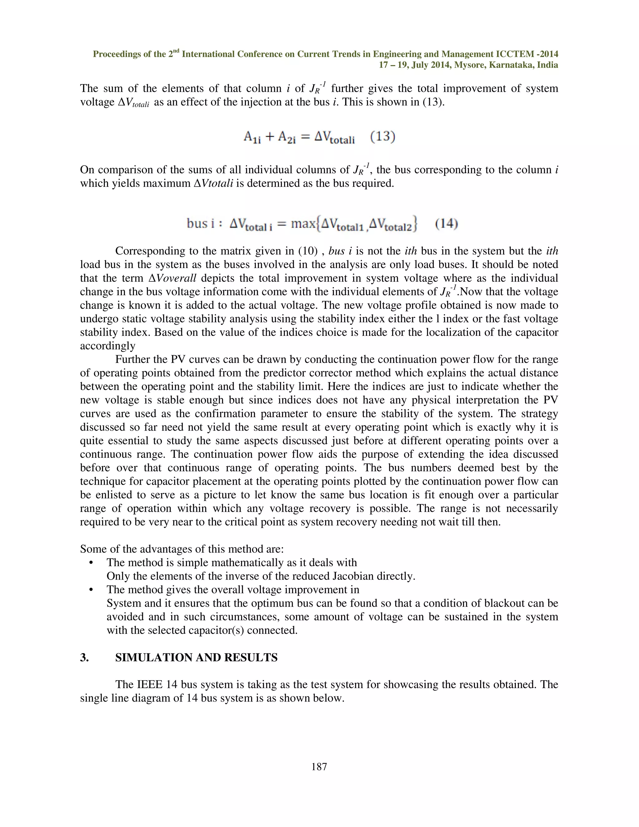
The idea of this paper is to point out the location (bus) capable of yielding the required
voltage improvement for the overall system, even if it doesn’t answer the exact amount of
compensation required. Main study in this paper involves injecting the unit amount of reactive power
into each bus which in turn enhance the voltage profile at all buses. The static voltage stability
analysis of the new voltage profile obtained at individual buses will count up to the basis of selecting
the location, which will better fit than the others.
The next section discusses the background of the technique, but they are noted in brief below:
• Conventional load flow analysis is performed using newton raphson technique
• The jacobian matrix is computed from conventional load flow. The reduced jacobian is
determined. The inverted jacobian is used to depict the change in the voltage in terms of
reactive power injection.
• This inverted jacobian is used in later section to determine the location where placing the
capacitor would yield maximum system voltage improvement.
• The voltage stability indices are used to perform the static voltage stability analysis for the new
183
voltage profile obtained
• The previous steps are repeated for a range of operating points using the continuation power
flow method and procedure is applied to each of these points.
The contribution of the proposed method lies in three major aspects firstly to determine the
capacitor location for the best overall improvement, secondly isolation of the locations which
are sure to not yield any significant improvement of the voltage and thirdly avoid the system
reaching the instability by monitoring the static stability of the system at subsequent operating
points. This procedure might turn out to be useful in situations where complete black out can be
avoided and scenario like a brownout can be improved towards the normal operating condition.
1. BACKGROUND THEORY
1.1 Computation of the reduced Jacobian
The jacobian obtained from newton raphson method is further reduced to evaluate the
suitable bus for placement of capacitors as shown in the next section. The reduced jacobian [1]
formulation is as shown below.
The matrix model of the load flow studies is given by](https://image.slidesharecdn.com/selectivelocalizationofcapacitorbanksconsideringstabilityaspectsinpowersystems-2-141006045653-conversion-gate01/75/Selective-localization-of-capacitor-banks-considering-stability-aspects-in-power-systems-2-2-2048.jpg)
![Proceedings of the 2nd International Conference on Current Trends in Engineering and Management ICCTEM -2014
17 – 19, July 2014, Mysore, Karnataka, India
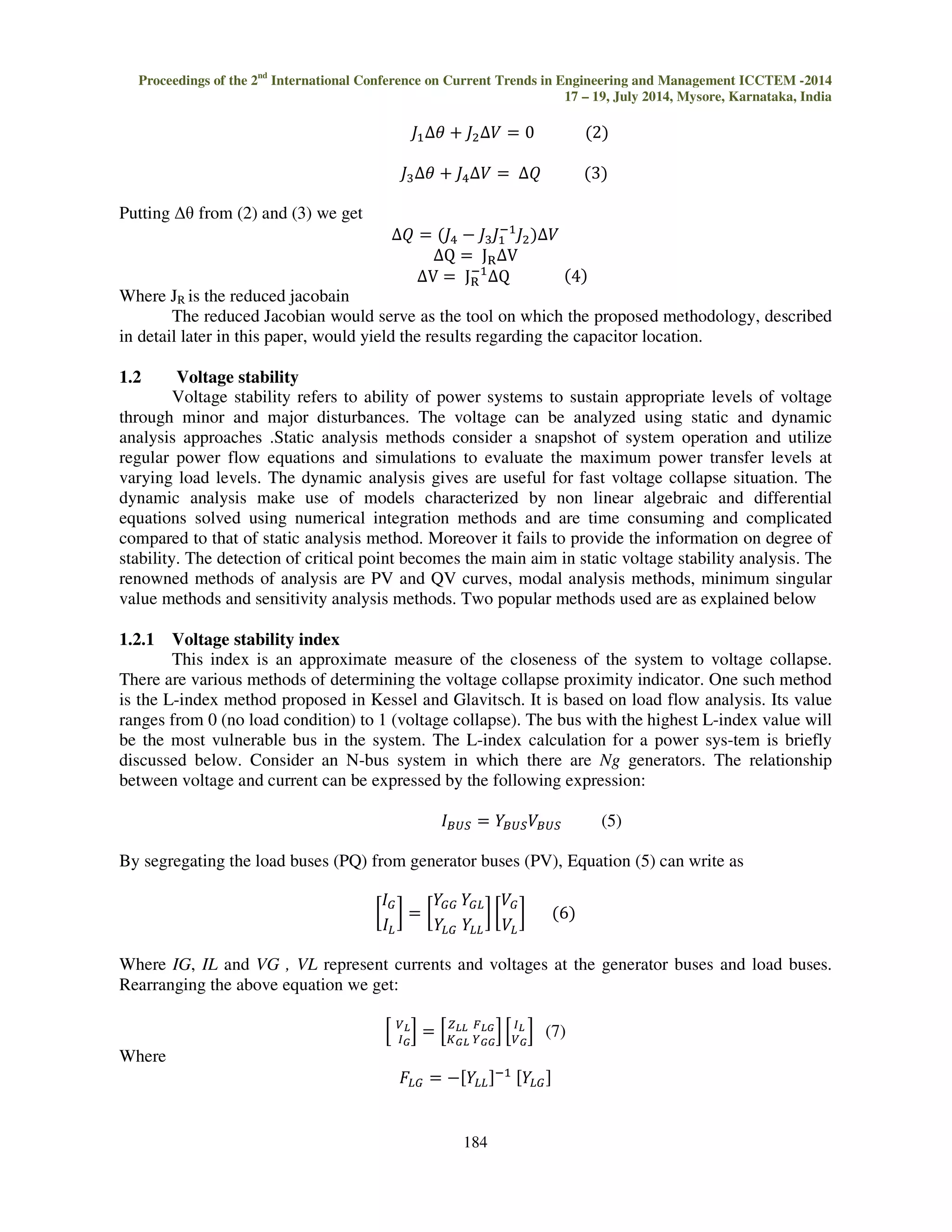
The L-index of the jth node is given by the expression:
185
?9 @ A
67 89 := ;7
A7 BC7 D D78 (8)
Where
Vi is the magnitude of the ith generator,
Vj is the voltage magnitude of the jth generator
ji is the phase angle of the term Fji
are the voltage phase angles of the generator units
Ng is the number of generating units
The values of Fji are obtained from the matrix FLG. The L-indices for a given load condition
are computed for all the load buses and the maximum of the L-indices (Lmax) gives the proximity of
the system to voltage collapse. The L-index has the advantage of indicating voltage in- stability
proximity of the current operating point without calculation of the information about the maximum
loading point.
Musirin has developed a line based stability index to indicate the stability of transmission
lines, which is termed as Fast Voltage Stability Index (FVSI). The FVSI of an l-th line can be
represented in as
3E!' F G
$H' I
Where Zl, Xl, Qr, and Vi are the line impedance, line reactance, receiving end power, and
sending end voltage respectively. It is important to note that for a stable power system, the FVSI
should be less than unity. Either of the indices is used for voltage stability analysis.
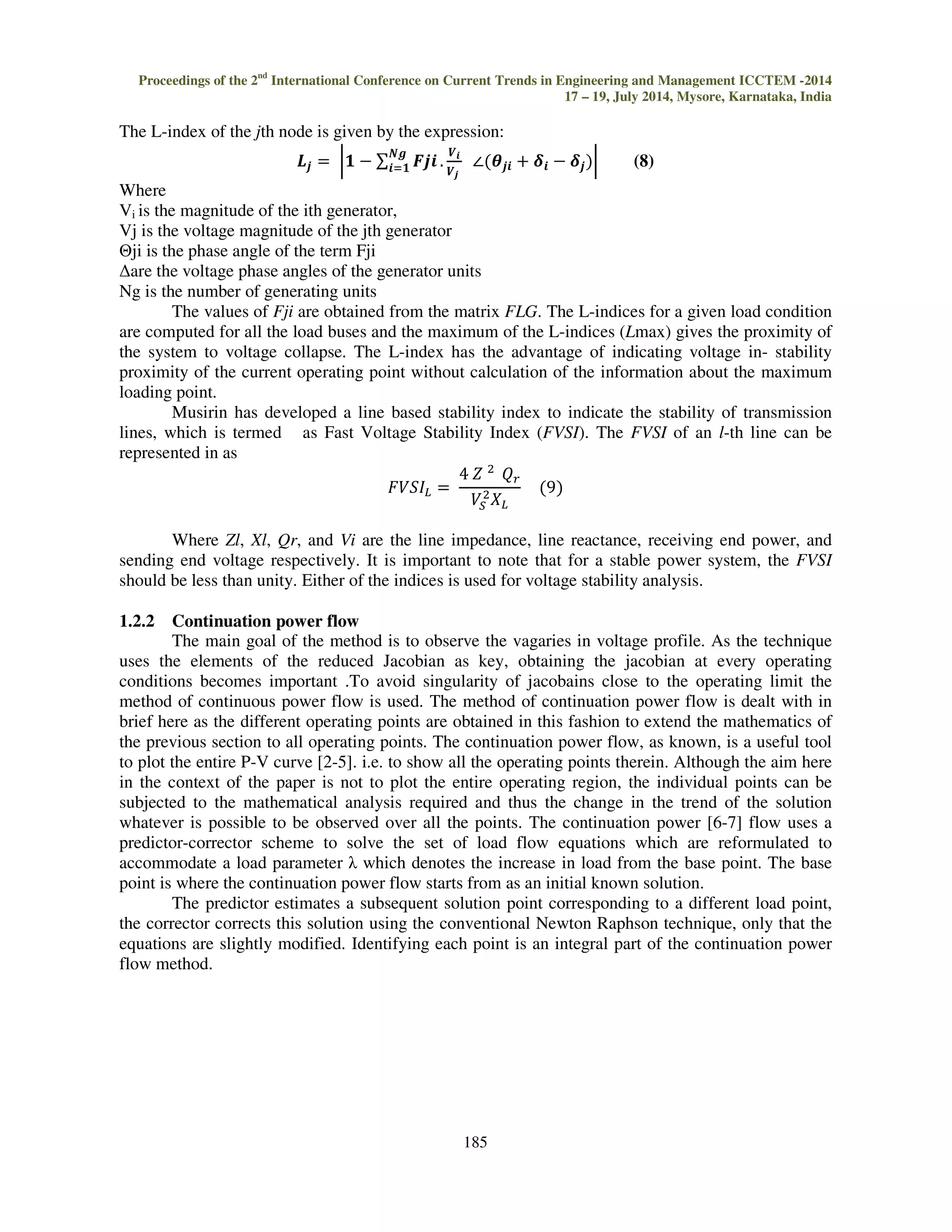
1.2.2 Continuation power flow
The main goal of the method is to observe the vagaries in voltage profile. As the technique
uses the elements of the reduced Jacobian as key, obtaining the jacobian at every operating
conditions becomes important .To avoid singularity of jacobains close to the operating limit the
method of continuous power flow is used. The method of continuation power flow is dealt with in
brief here as the different operating points are obtained in this fashion to extend the mathematics of
the previous section to all operating points. The continuation power flow, as known, is a useful tool
to plot the entire P-V curve [2-5]. i.e. to show all the operating points therein. Although the aim here
in the context of the paper is not to plot the entire operating region, the individual points can be
subjected to the mathematical analysis required and thus the change in the trend of the solution
whatever is possible to be observed over all the points. The continuation power [6-7] flow uses a
predictor-corrector scheme to solve the set of load flow equations which are reformulated to
accommodate a load parameter which denotes the increase in load from the base point. The base
point is where the continuation power flow starts from as an initial known solution.
The predictor estimates a subsequent solution point corresponding to a different load point,
the corrector corrects this solution using the conventional Newton Raphson technique, only that the
equations are slightly modified. Identifying each point is an integral part of the continuation power
flow method.](https://image.slidesharecdn.com/selectivelocalizationofcapacitorbanksconsideringstabilityaspectsinpowersystems-2-141006045653-conversion-gate01/75/Selective-localization-of-capacitor-banks-considering-stability-aspects-in-power-systems-2-7-2048.jpg)
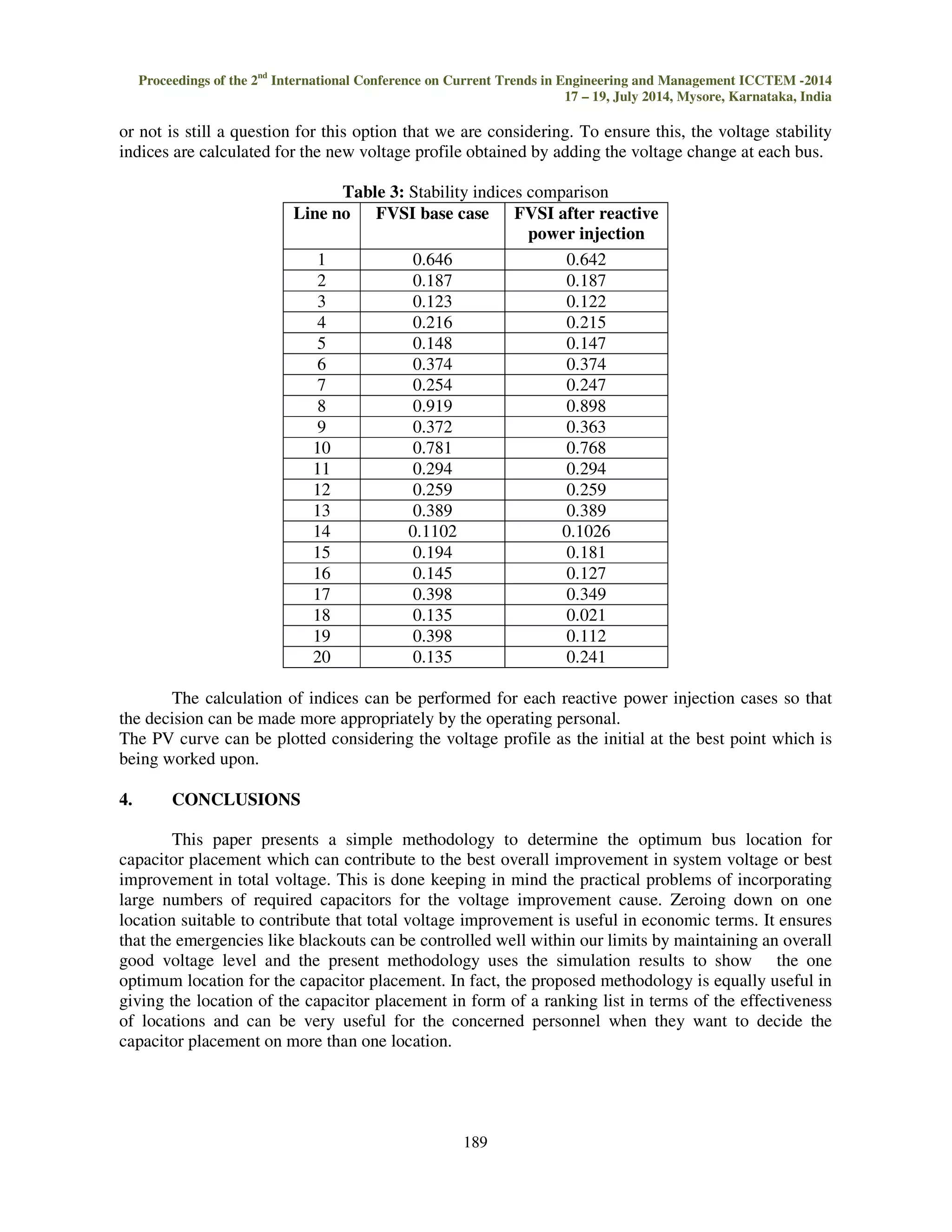


This document presents a methodology for determining optimal locations for capacitor bank placement to enhance voltage stability in power systems. It discusses the significance of voltage stability in interconnected systems and employs static voltage stability analysis, using a reduced Jacobian method to identify ideal bus positions for reactive power injection. Results demonstrate that injecting reactive power at bus 14 yields the highest overall voltage improvement, suggesting it as a key location for capacitor installation.


![Vibe Coding vs. Spec-Driven Development [Free Meetup]](https://cdn.slidesharecdn.com/ss_thumbnails/vibecodingvsspecdrivendevelopment-251209105622-43f455e7-thumbnail.jpg?width=640&height=640&fit=bounds)


