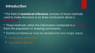
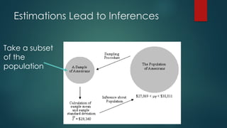
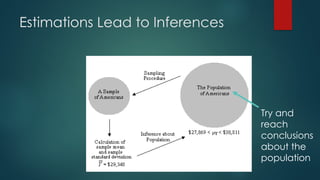
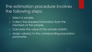
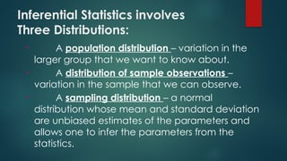
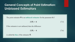
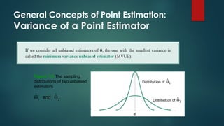
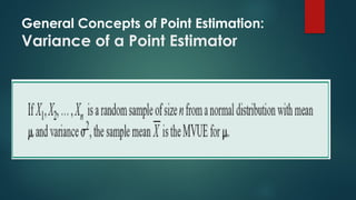
SAMPLING DISTRIBUTION AND
POINT ESTIMATION OF
PARAMETERS
Introduction
• The field of statistical inference consists of those methods
used to make decisions or to draw conclusions about a
population.
• These methods utilize the information contained in a sample
from the population in drawing conclusions.
• Statistical inference may be divided into two major areas:
• Parameter estimation
• Hypothesis testing
ESTIMATION
A process whereby we select a random
sample from a population and use a
sample statistic to estimate a population
parameter.
EXAMPLES OF ESTIMATION
 an auto company may want to estimate the mean
fuel consumption for a particular model of a car
 a manager may want to estimate the average time
taken by new employees to learn a job;
 the U.S. Census Bureau may want to find the mean
housing expenditure per month incurred by
households;
 and the AWAH (Association of Wives of Alcoholic
Husbands) may want to find the proportion (or
percentage) of all husbands who are alcoholic.
Take a subset
of the
population
Estimations Lead to Inferences
Try and
reach
conclusions
about the
population
The estimation procedure involves
the following steps:
1. Select a sample.
2. Collect the required information from the
members of the sample.
3. Calculate the value of the sample statistic.
4. Assign value(s) to the corresponding population
parameter.
Inferential Statistics involves
Three Distributions:
• A population distribution – variation in the
larger group that we want to know about.
• A distribution of sample observations –
variation in the sample that we can observe.
• A sampling distribution – a normal
distribution whose mean and standard deviation
are unbiased estimates of the parameters and
allows one to infer the parameters from the
statistics.
ESTIMATION
ESTIMATION
POINT ESTIMATION
A sample statistic is used to estimate the exact value
of a population parameter.
Point Estimator
A point estimator draws inference
about a population by estimating the
value of an unknown parameter using
a single value or a point.
Sampling Distributions and the Central
Limit Theorem
Statistical inference is concerned with making decisions about a
population based on the information contained in a random
sample from that population.
Definitions:
THE CENTRAL LIMIT THEOREM
 As the sample size n increases without limit, the
shape of the distribution of the sample means
taken with replacement from a population with
mean µ and standard deviation σ will approach
a normal distribution. As previously shown, this
distribution will have a mean µ and a standard
deviation σ /√n.
7.2 Sampling Distributions and the
Central Limit Theorem
Figure 7-1
Distributions of
average scores from
throwing dice.
[Adapted with
permission from
Box, Hunter, and
Hunter (1978). ]
Sampling Distributions and the Central
Limit Theorem
Procedure Table
1. Draw a normal curve and shade the desired
area.
2. Convert the X value to a z value.
3. Find the corresponding area for the z value.
Sampling Distributions and the
Central Limit Theorem
It’s important to remember two things when you use the central
limit theorem:
1. When the original variable is normally distributed, the
distribution of the sample means will be normally distributed,
for any sample size n.
2. When the distribution of the original variable is not normal, a
sample size of 30 or more is needed to use a normal
distribution to approximate the distribution of the sample
means. The larger the sample, the better the approximation
will be.
Sampling Distributions and the
Central Limit Theorem
1. An electronics company manufactures resistors that
have a mean resistance of 100 ohms and a standard
deviation of 10 ohms. The distribution of resistance is
normal. Find the probability that a random sample of n
= 25 resistors will have an average resistance less than 95
ohms.
Sampling Distributions and the
Central Limit Theorem
2. A. C. Neilsen reported that children between
the ages of 2 and 5 watch an average of 25 hours
of television per week. Assume the variable is
normally distributed and the standard deviation is
3 hours. If 20 children between the ages of 2 and 5
are randomly selected, find the probability that
the mean of the number of hours they watch
television will be greater than 26.3 hours.
Sampling Distributions and the
Central Limit Theorem
3. The average time spent by construction workers
who work on weekends is 7.93 hours (over 2 days).
Assume the distribution is approximately normal
and has a standard deviation of 0.8 hour. If a
sample of 40 construction workers is randomly
selected, find the probability that the mean of the
sample will be less than 8 hours.
Sampling Distributions and the
Central Limit Theorem
4. The average age of a vehicle registered in the
United States is 8 years, or 96 months. Assume the
standard deviation is 16 months. If a random
sample of 36 vehicles is selected, find the
probability that the mean of their age is between
90 and 100 months.
Sampling Distributions and the
Central Limit Theorem
Approximate Sampling Distribution of a Difference in
Sample Means
General Concepts of Point Estimation:
Unbiased Estimators
What can I do to Ensure Unbiasedness in my Data or
Sampling Distribution?
 Take your sample according to sound statistical
practices.
 Avoid measurement error by making sure data is
collected with unbiased practices. For example,
make sure any questions posed aren’t ambiguous.
 Avoid unrepresentative samples by making sure
you haven’t excluded certain population members
(like minorities or people who work two jobs).
General Concepts of Point Estimation:
Variance of a Point Estimator
Figure 7-5 The sampling
distributions of two unbiased
estimators
.
ˆ
ˆ
2
1 
 and
General Concepts of Point Estimation:
Variance of a Point Estimator
General Concepts of Point Estimation: Standard
Error: Reporting a Point Estimate
General Concepts of Point Estimation: Standard
Error: Reporting a Point Estimate
General Concepts of Point Estimation:
Mean Square Error of an Estimator
General Concepts of Point Estimation:
Mean Square Error of an Estimator
General Concepts of Point Estimation:
Mean Square Error of an Estimator
Figure 7-6 A biased estimator that has smaller variance than the unbiased
estimator
1
̂
.
ˆ
2

Three Properties of a Good
Estimator
1. The estimator should be an unbiased estimator. That is, the
expected value or the mean of the estimates obtained from
samples of a given size is equal to the parameter being
estimated.
2. The estimator should be consistent. For a consistent
estimator, as sample size increases, the value of the
estimator approaches the value of the parameter
estimated.
3. The estimator should be a relatively efficient estimator. That
is, of all the statistics that can be used to estimate a
parameter, the relatively efficient estimator has the smallest
variance.

SAMPLING DISTRIBUTION AND POINT ESTIMATION OF PARAMETERS - Copy.pptx

  • 1.
    SAMPLING DISTRIBUTION AND POINTESTIMATION OF PARAMETERS
  • 2.
    Introduction • The fieldof statistical inference consists of those methods used to make decisions or to draw conclusions about a population. • These methods utilize the information contained in a sample from the population in drawing conclusions. • Statistical inference may be divided into two major areas: • Parameter estimation • Hypothesis testing
  • 3.
    ESTIMATION A process wherebywe select a random sample from a population and use a sample statistic to estimate a population parameter.
  • 4.
    EXAMPLES OF ESTIMATION an auto company may want to estimate the mean fuel consumption for a particular model of a car  a manager may want to estimate the average time taken by new employees to learn a job;  the U.S. Census Bureau may want to find the mean housing expenditure per month incurred by households;  and the AWAH (Association of Wives of Alcoholic Husbands) may want to find the proportion (or percentage) of all husbands who are alcoholic.
  • 5.
    Take a subset ofthe population Estimations Lead to Inferences
  • 6.
    Estimations Lead toInferences Try and reach conclusions about the population
  • 7.
    The estimation procedureinvolves the following steps: 1. Select a sample. 2. Collect the required information from the members of the sample. 3. Calculate the value of the sample statistic. 4. Assign value(s) to the corresponding population parameter.
  • 8.
    Inferential Statistics involves ThreeDistributions: • A population distribution – variation in the larger group that we want to know about. • A distribution of sample observations – variation in the sample that we can observe. • A sampling distribution – a normal distribution whose mean and standard deviation are unbiased estimates of the parameters and allows one to infer the parameters from the statistics.
  • 9.
  • 10.
  • 11.
    POINT ESTIMATION A samplestatistic is used to estimate the exact value of a population parameter.
  • 12.
    Point Estimator A pointestimator draws inference about a population by estimating the value of an unknown parameter using a single value or a point.
  • 13.
    Sampling Distributions andthe Central Limit Theorem Statistical inference is concerned with making decisions about a population based on the information contained in a random sample from that population. Definitions:
  • 14.
    THE CENTRAL LIMITTHEOREM  As the sample size n increases without limit, the shape of the distribution of the sample means taken with replacement from a population with mean µ and standard deviation σ will approach a normal distribution. As previously shown, this distribution will have a mean µ and a standard deviation σ /√n.
  • 15.
    7.2 Sampling Distributionsand the Central Limit Theorem Figure 7-1 Distributions of average scores from throwing dice. [Adapted with permission from Box, Hunter, and Hunter (1978). ]
  • 16.
    Sampling Distributions andthe Central Limit Theorem
  • 17.
    Procedure Table 1. Drawa normal curve and shade the desired area. 2. Convert the X value to a z value. 3. Find the corresponding area for the z value.
  • 18.
    Sampling Distributions andthe Central Limit Theorem It’s important to remember two things when you use the central limit theorem: 1. When the original variable is normally distributed, the distribution of the sample means will be normally distributed, for any sample size n. 2. When the distribution of the original variable is not normal, a sample size of 30 or more is needed to use a normal distribution to approximate the distribution of the sample means. The larger the sample, the better the approximation will be.
  • 19.
    Sampling Distributions andthe Central Limit Theorem 1. An electronics company manufactures resistors that have a mean resistance of 100 ohms and a standard deviation of 10 ohms. The distribution of resistance is normal. Find the probability that a random sample of n = 25 resistors will have an average resistance less than 95 ohms.
  • 20.
    Sampling Distributions andthe Central Limit Theorem 2. A. C. Neilsen reported that children between the ages of 2 and 5 watch an average of 25 hours of television per week. Assume the variable is normally distributed and the standard deviation is 3 hours. If 20 children between the ages of 2 and 5 are randomly selected, find the probability that the mean of the number of hours they watch television will be greater than 26.3 hours.
  • 21.
    Sampling Distributions andthe Central Limit Theorem 3. The average time spent by construction workers who work on weekends is 7.93 hours (over 2 days). Assume the distribution is approximately normal and has a standard deviation of 0.8 hour. If a sample of 40 construction workers is randomly selected, find the probability that the mean of the sample will be less than 8 hours.
  • 22.
    Sampling Distributions andthe Central Limit Theorem 4. The average age of a vehicle registered in the United States is 8 years, or 96 months. Assume the standard deviation is 16 months. If a random sample of 36 vehicles is selected, find the probability that the mean of their age is between 90 and 100 months.
  • 23.
    Sampling Distributions andthe Central Limit Theorem Approximate Sampling Distribution of a Difference in Sample Means
  • 24.
    General Concepts ofPoint Estimation: Unbiased Estimators
  • 25.
    What can Ido to Ensure Unbiasedness in my Data or Sampling Distribution?  Take your sample according to sound statistical practices.  Avoid measurement error by making sure data is collected with unbiased practices. For example, make sure any questions posed aren’t ambiguous.  Avoid unrepresentative samples by making sure you haven’t excluded certain population members (like minorities or people who work two jobs).
  • 26.
    General Concepts ofPoint Estimation: Variance of a Point Estimator Figure 7-5 The sampling distributions of two unbiased estimators . ˆ ˆ 2 1   and
  • 27.
    General Concepts ofPoint Estimation: Variance of a Point Estimator
  • 28.
    General Concepts ofPoint Estimation: Standard Error: Reporting a Point Estimate
  • 29.
    General Concepts ofPoint Estimation: Standard Error: Reporting a Point Estimate
  • 30.
    General Concepts ofPoint Estimation: Mean Square Error of an Estimator
  • 31.
    General Concepts ofPoint Estimation: Mean Square Error of an Estimator
  • 32.
    General Concepts ofPoint Estimation: Mean Square Error of an Estimator Figure 7-6 A biased estimator that has smaller variance than the unbiased estimator 1 ̂ . ˆ 2 
  • 33.
    Three Properties ofa Good Estimator 1. The estimator should be an unbiased estimator. That is, the expected value or the mean of the estimates obtained from samples of a given size is equal to the parameter being estimated. 2. The estimator should be consistent. For a consistent estimator, as sample size increases, the value of the estimator approaches the value of the parameter estimated. 3. The estimator should be a relatively efficient estimator. That is, of all the statistics that can be used to estimate a parameter, the relatively efficient estimator has the smallest variance.

Editor's Notes

  • #2 Statistical inference is the process by which we acquire information about populations from samples. There are two procedures for making inferences: Estimation. Hypotheses testing.
  • #3 The objective of estimation is to determine the value of a population parameter on the basis of a sample statistic. There are two types of estimators Point Estimator Interval estimator
  • #4 Estimate and Estimator The value(s) assigned to a population parameter based on the value of a sample statistic is called an estimate. The sample statistic used to estimate a population parameter is called an estimator.
  • #11 A point estimator draws inference about a population by estimating the value of an unknown parameter using a single value or a point.
  • #16 If the sample size is sufficiently large, the central limit theorem can be used to answer questions about sample means in the same manner that a normal distribution can be used to answer questions about individual values. The only difference is that a new formula must be used for the z values. It is If a large number of samples of a given size are selected from a normally distributed population, or if a large number of samples of a given size that is greater than or equal to 30 are selected from a population that is not normally distributed, and the sample means are computed, then the distribution of sample means will look like the one shown in Figure 6–33. Their percentages indicate the areas of the regions.
  • #24 An unbiased estimator is one that produces the right answer on average. Bias occurs when there is a systematic error in the measure that shifts the estimate more in one direction than another over a set of replications. In general, we can consider any population parameter, , and denote its estimator by U. U is an unbiased estimator of  if E(U) = . Any bias that occurs is Bias = E(V) - . To avoid bias, we should randomly sample from the whole population. KKV note that one form of bias that is common in the social sciences is due to people that are wary of providing information that we need for our analyses (study of education in India). Other examples of systematic bias: race/interviewer effects, acquiescence bias, response bias An unbiased estimator is an accurate statistic that’s used to approximate a population parameter. “Accurate” in this sense means that it’s neither an overestimate nor an underestimate. If an overestimate or underestimate does happen, the mean of the difference is called a “bias.”
  • #25 There are many steps you can take to try and make sure that your statistics are unbiased and accurately reflect the population parameter you are studying: For more information on different sampling types and the advantages and disadvantages of each, see: Sampling Techniques
  • #26 As well as being on target on the average, we would also like the distribution of an estimator to be highly concentrated, that is, to have a small variance. This is the notion of efficiency. Efficiency of V compared to W = var W/var V where V and W are two estimators, such as the mean and median How do we increase efficiency? We know that more observations will produce more efficient estimators because the standard error of most of the sampling distributions we have discussed involve dividing by n.
  • #27 For normal populations, the efficiency of the mean relative to the median is equal to 1.57. This means that the mean is about 57% more efficient than the sample median. Efficiency is a way generally of comparing unbiased estimators, but KKV (pages 70-74) show that you can use the same criteria to compare estimators with a small amount of bias; sometimes you would prefer a more efficient estimator with a small amount of bias to a unbiased estimator that is not efficient. In comparing unbiased estimators, we choose the one with minimum variance. Figure 7-3 (page 239) shows some examples of unbiased estimates that might be inefficient and biased estimates that might be more efficient. Statisticians use both criteria for determining good estimators. They use the Mean Square Error or MSE = E(V - )2 = variance of estimator + (its bias)2. We choose the estimator that minimizes this MSE.
  • #30 The property of consistency is such that as the number of observations gets very large, the variability around your estimate decreases to zero, and the estimate equals the parameter we are trying to estimate. One of the conditions that makes an estimator consistent is if its bias and variance both approach zero. In other words, we expect the MSE to approach zero in the limit.