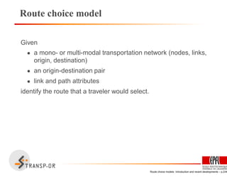
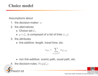
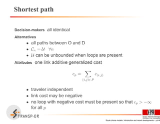
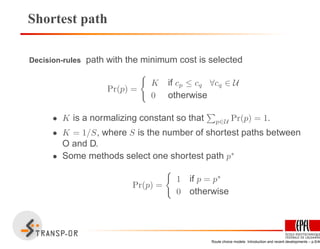
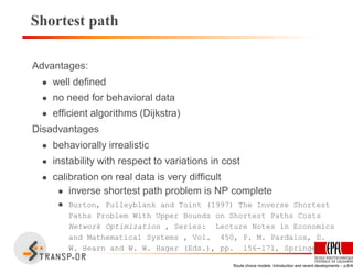
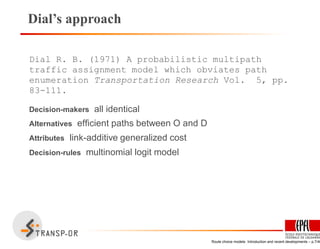
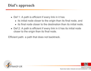
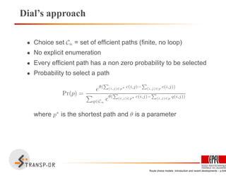
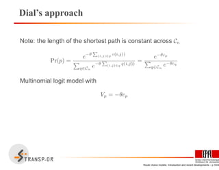
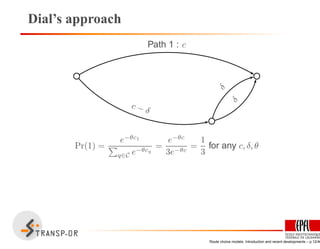
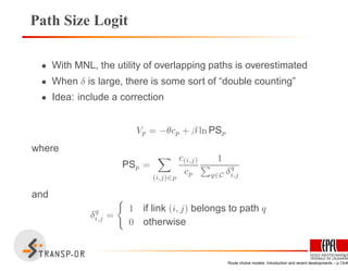
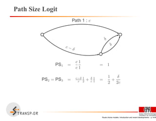
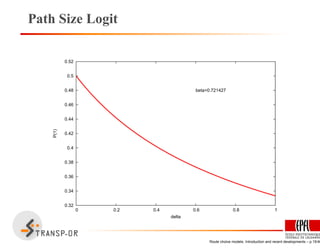
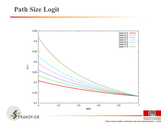
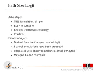
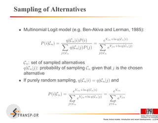
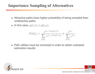
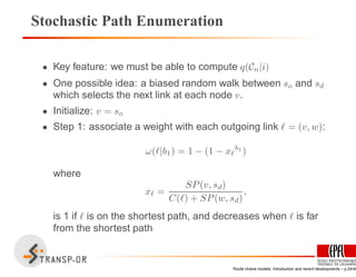
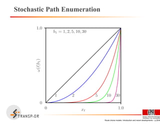
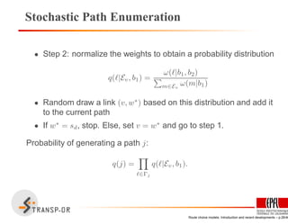
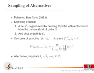
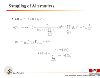
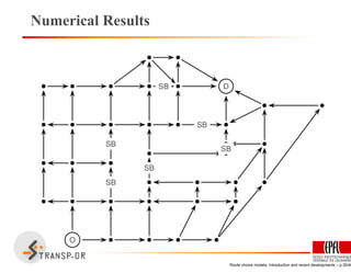
This document discusses route choice models and recent developments in the field. It introduces the basic components of a route choice model, including a transportation network, origin-destination pairs, link and path attributes. It then describes several classic models: the shortest path model, Dial's approach using a multinomial logit model on efficient paths, and the path size logit which addresses issues with overlapping paths in the multinomial logit. The document also discusses challenges with path enumeration and different approaches to address this such as stochastic path generation and sampling of alternatives from the universal set of paths.

1. Route choice models: Introduction and recent
developments
Michel Bierlaire
transp-or.epfl.ch
Transport and Mobility Laboratory, EPFL
Route choice models: Introduction and recent developments – p.1/40

2. Route choice model
Given
• a mono- or multi-modal transportation network (nodes, links,
origin, destination)
• an origin-destination pair
• link and path attributes
identify the route that a traveler would select.
Route choice models: Introduction and recent developments – p.2/40

3. Choice model
Assumptions about
1. the decision-maker: n
2. the alternatives
• Choice set Cn
• p ∈ Cn is composed of a list of links (i, j)
3. the attributes
• link-additive: length, travel time, etc.
xkp =
(i,j)∈P
xk(i,j)
• non link-additive: scenic path, usual path, etc.
4. the decision-rules: Pr(p|Cn)
Route choice models: Introduction and recent developments – p.3/40

4. Shortest path
Decision-makers all identical
Alternatives
• all paths between O and D
• Cn = U ∀n
• U can be unbounded when loops are present
Attributes one link additive generalized cost
cp =
(i,j)∈P
c(i,j)
• traveler independent
• link cost may be negative
• no loop with negative cost must be present so that cp > −∞
for all p
Route choice models: Introduction and recent developments – p.4/40

5. Shortest path
Decision-rules path with the minimum cost is selected
Pr(p) =
K if cp ≤ cq ∀cq ∈ U
0 otherwise
• K is a normalizing constant so that p∈U Pr(p) = 1.
• K = 1/S, where S is the number of shortest paths between
O and D.
• Some methods select one shortest path p∗
Pr(p) =
1 if p = p∗
0 otherwise
Route choice models: Introduction and recent developments – p.5/40

6. Shortest path
Advantages:
• well defined
• no need for behavioral data
• efficient algorithms (Dijkstra)
Disadvantages
• behaviorally irrealistic
• instability with respect to variations in cost
• calibration on real data is very difficult
• inverse shortest path problem is NP complete
• Burton, Pulleyblank and Toint (1997) The Inverse Shortest
Paths Problem With Upper Bounds on Shortest Paths Costs
Network Optimization , Series: Lecture Notes in Economics
and Mathematical Systems , Vol. 450, P. M. Pardalos, D.
W. Hearn and W. W. Hager (Eds.), pp. 156-171, Springer
Route choice models: Introduction and recent developments – p.6/40

7. Dial’s approach
Dial R. B. (1971) A probabilistic multipath
traffic assignment model which obviates path
enumeration Transportation Research Vol. 5, pp.
83-111.
Decision-makers all identical
Alternatives efficient paths between O and D
Attributes link-additive generalized cost
Decision-rules multinomial logit model
Route choice models: Introduction and recent developments – p.7/40

8. Dial’s approach
• Def 1: A path is efficient if every link in it has
• its initial node closer to the origin than its final node, and
• its final node closer to the destination than its initial node.
• Def 2: A path is efficient if every link in it has its initial node
closer to the origin than its final node.
Efficient path: a path that does not backtrack.
Route choice models: Introduction and recent developments – p.8/40

9. Dial’s approach
• Choice set Cn = set of efficient paths (finite, no loop)
• No explicit enumeration
• Every efficient path has a non zero probability to be selected
• Probability to select a path
Pr(p) =
eθ(
P
(i,j)∈p∗ c(i,j)−
P
(i,j)∈p c(i,j))
q∈Cn
eθ(
P
(i,j)∈p∗ c(i,j)−
P
(i,j)∈p q(i,j))
where p∗
is the shortest path and θ is a parameter
Route choice models: Introduction and recent developments – p.9/40

10. Dial’s approach
Note: the length of the shortest path is constant across Cn
Pr(p) =
e−θ
P
(i,j)∈p c(i,j))
q∈Cn
e−θ
P
(i,j)∈q q(i,j))
=
e−θcp
q∈Cn
e−θcq
Multinomial logit model with
Vp = −θcp
Route choice models: Introduction and recent developments – p.10/40

11. Dial’s approach
Advantages:
• probabilistic model, more stable
• calibration parameter θ
• avoid path enumeration
• designed for traffic assignment
Disadvantages:
• MNL assumes independence among alternatives
• efficient paths are mathematically convenient but not
behaviorally motivated
Route choice models: Introduction and recent developments – p.11/40

12. Dial’s approach
Path 1 : c
c − δ
δ
δ
Pr(1) =
e−θc1
q∈C e−θcq
=
e−θc
3e−θc
=
1
3
for any c, δ, θ
Route choice models: Introduction and recent developments – p.12/40

13. Path Size Logit
• With MNL, the utility of overlapping paths is overestimated
• When δ is large, there is some sort of “double counting”
• Idea: include a correction
Vp = −θcp + β ln PSp
where
PSp =
(i,j)∈p
c(i,j)
cp
1
q∈C δq
i,j
and
δq
i,j =
1 if link (i, j) belongs to path q
0 otherwise
Route choice models: Introduction and recent developments – p.13/40

14. Path Size Logit
Path 1 : c
c − δ
δ
δ
PS1 =
c
c
1
1
= 1
PS2 = PS3 = c−δ
c
1
2 + δ
c
1
1 =
1
2
+
δ
2c
Route choice models: Introduction and recent developments – p.14/40

15. Path Size Logit
0.32
0.34
0.36
0.38
0.4
0.42
0.44
0.46
0.48
0.5
0.52
0 0.2 0.4 0.6 0.8 1
P(1)
delta
beta=0.721427
Route choice models: Introduction and recent developments – p.15/40

16. Path Size Logit
0.3
0.35
0.4
0.45
0.5
0.55
0.6
0.65
0 0.2 0.4 0.6 0.8 1
P(1)
delta
beta=0.4
beta=0.5
beta=0.6
beta=0.7
beta=0.8
beta=0.9
beta=1.0
Route choice models: Introduction and recent developments – p.16/40

17. Path Size Logit
Advantages:
• MNL formulation: simple
• Easy to compute
• Exploits the network topology
• Practical
Disadvantages:
• Derived from the theory on nested logit
• Several formulations have been proposed
• Correlated with observed and unobserved attributes
• May give biased estimates
Route choice models: Introduction and recent developments – p.17/40

18. Path Size Logit: readings
• Cascetta, E., Nuzzolo, A., Russo, F., Vitetta,
A. 1996. A modified logit route choice model
overcoming path overlapping problems.
Specification and some calibration results for
interurban networks. In Lesort, J.B. (Ed.),
Proceedings of the 13th International Symposium
on Transportation and Traffic Theory, Lyon,
France.
• Ramming, M., 2001. Network Knowledge and Route
Choice, PhD thesis, Massachusetts Institute of
Technology.
• Ben-Akiva, M., and Bierlaire, M. (2003).
Discrete choice models with applications to
departure time and route choice. In Hall, R.
(ed) Handbook of Transportation Science, 2nd
edition pp.7-38. Kluwer.
Route choice models: Introduction and recent developments – p.18/40

19. Path Size Logit: readings
• Hoogendoorn-Lanser, S., van Nes, R. and Bovy,
P. (2005) Path Size Modeling in Multimodal
Route Choice Analysis. Transportation Research
Record vol. 1921 pp. 27-34
• Frejinger, E., and Bierlaire, M. (2007).
Capturing correlation with subnetworks in route
choice models, Transportation Research Part B:
Methodological 41(3):363-378.
doi:10.1016/j.trb.2006.06.003
Route choice models: Introduction and recent developments – p.19/40

20. Path enumeration
• Dial’s approach avoids path enumeration
• Computationally convenient but behaviorally incorrect
• MNL inappropriate due to significant path overlap
• Generalized cost must be link-additive
• Heterogeneity in terms of behavior, equipments, etc. cannot be
accounted for.
• With other DCM models, choice sets must be explicitly defined
• Path enumeration heuristics have been proposed:
• Deterministic approaches: link elimination (Azevedo et al.,
1993), labeled paths (Ben-Akiva et al., 1984)
• Stochastic approaches: simulation (Ramming, 2001) and
doubly stochastic (Bovy and Fiorenzo-Catalano, 2006)
Route choice models: Introduction and recent developments – p.20/40

21. Path enumeration
• Underlying assumption in existing approaches: the actual
choice set is generated
• Empirical results suggest that this is not always true
• Our approach:
• Choice set contains all paths
• Too large for computation
• Solution: sampling of alternatives
Route choice models: Introduction and recent developments – p.21/40

22. Sampling of Alternatives
• Multinomial Logit model (e.g. Ben-Akiva and Lerman, 1985):
P(i|Cn) =
q(Cn|i)P(i)
j∈Cn
q(Cn|j)P(j)
=
eVin+ln q(Cn|i)
j∈Cn
eVjn+ln q(Cn|j)
Cn: set of sampled alternatives
q(Cn|j): probability of sampling Cn given that j is the chosen
alternative
• If purely random sampling, q(Cn|i) = q(Cn|j) and
P(i|Cn) =
eVin+ln q(Cn|i)
j∈Cn
eVjn+ln q(Cn|j)
=
eVin
j∈Cn
eVjn
Route choice models: Introduction and recent developments – p.22/40

23. Importance Sampling of Alternatives
• Attractive paths have higher probability of being sampled than
unattractive paths
• In this case, q(Cn|i) = q(Cn|j)
P(i|Cn) =
eVin+ln q(Cn|i)
j∈Cn
eVjn+ln q(Cn|j)
=
eVin
j∈Cn
eVjn
• Path utilities must be corrected in order to obtain unbiased
estimation results
Route choice models: Introduction and recent developments – p.23/40

24. Stochastic Path Enumeration
• Key feature: we must be able to compute q(Cn|i)
• One possible idea: a biased random walk between so and sd
which selects the next link at each node v.
• Initialize: v = so
• Step 1: associate a weight with each outgoing link ℓ = (v, w):
ω(ℓ|b1) = 1 − (1 − xℓ
b1
)
where
xℓ =
SP(v, sd)
C(ℓ) + SP(w, sd)
,
is 1 if ℓ is on the shortest path, and decreases when ℓ is far
from the shortest path
Route choice models: Introduction and recent developments – p.24/40

25. Stochastic Path Enumeration
0 1.0
0
1.0
xℓ
ω(ℓ|b1)
1 2 5 10 30
b1 = 1, 2, 5, 10, 30
Route choice models: Introduction and recent developments – p.25/40

26. Stochastic Path Enumeration
• Step 2: normalize the weights to obtain a probability distribution
q(ℓ|Ev, b1) =
ω(ℓ|b1, b2)
m∈Ev
ω(m|b1)
• Random draw a link (v, w∗
) based on this distribution and add it
to the current path
• If w∗
= sd, stop. Else, set v = w∗
and go to step 1.
Probability of generating a path j:
q(j) =
ℓ∈Γj
q(ℓ|Ev, b1).
Route choice models: Introduction and recent developments – p.26/40

27. Sampling of Alternatives
• Following Ben-Akiva (1993)
• Sampling protocol
1. A set Cn is generated by drawing R paths with replacement
from the universal set of paths U
2. Add chosen path to Cn
• Outcome of sampling: (k1, k2, . . . , kJ ) and J
j=1 kj = R
P(k1, k2, . . . , kJ ) =
R!
j∈U kj! j∈U
q(j)
ekj
• Alternative j appears kj = kj + δcj in Cn
Route choice models: Introduction and recent developments – p.27/40

28. Sampling of Alternatives
• Let Cn = {j ∈ U | kj > 0}
q(Cn|i) = q(Cn|i) =
R!
(ki − 1)!
j∈Cn
j=i
kj!
q(i)ki−1
j∈Cn
j=i
q(j)kj
= KCn
ki
q(i)
KCn = R!Q
j∈Cn
kj ! j∈Cn
q(j)kj
P(i|Cn) =
e
Vin+ln
“
ki
q(i)
”
j∈Cn
e
Vjn+ln
“ kj
q(j)
”
Route choice models: Introduction and recent developments – p.28/40

29. Numerical Results
• Estimation of models based on synthetic data generated with a
postulated model
• Evaluation of
• Sampling correction
• Path Size attribute
• Biased random walk algorithm parameters
Route choice models: Introduction and recent developments – p.29/40

30. Numerical Results
O
D
SB
SB
SB
SB
SB
SB
Route choice models: Introduction and recent developments – p.30/40

31. Numerical Results
• True model: Path Size Logit
Uj = βPS ln PSU
j + βLLengthj + βSBSpeedBumpsj + εj
βPS = 1, βL = −0.3, βSB = −0.1
εj distributed Extreme Value with scale 1 and location 0
PSU
j = ℓ∈Γj
Lℓ
Lj
1P
p∈U δℓp
• 3000 observations
Route choice models: Introduction and recent developments – p.31/40

32. Numerical Results
• Four model specifications
Sampling Correction
Without With
Path
Size
C MNoCorr
P S(C) MCorr
P S(C)
U MNoCorr
P S(U) MCorr
P S(U)
PSU
i = ℓ∈Γi
Lℓ
Li
1P
j∈U δℓj
PSC
in = ℓ∈Γi
Lℓ
Li
1P
j∈Cn
δℓj
Route choice models: Introduction and recent developments – p.32/40

33. Numerical Results
• Model MNoCorr
P S(C) :
Vin = µ
“
βPS ln PSC
in − 0.3Lengthi + βSBSpeedBumpsi
”
• Model MCorr
P S(C):
Vin = µ
“
βPS ln PSC
in − 0.3Lengthi + βSBSpeedBumpsi
”
+ ln( ki
q(i)
)
• Model MNoCorr
P S(U) :
Vin = µ
“
βPS ln PSU
in − 0.3Lengthi + βSBSpeedBumpsi
”
• Model MCorr
P S(U):
Vin = µ
“
βPS ln PSU
in − 0.3Lengthi + βSBSpeedBumpsi
”
+ ln( ki
q(i)
)
Route choice models: Introduction and recent developments – p.33/40

34. Numerical Results
True MNoCorr
P S(C)
MCorr
P S(C)
MNoCorr
P S(U)
MCorr
P S(U)
PSL PSL PSL PSL PSL
βL fixed -0.3 -0.3 -0.3 -0.3 -0.3
bµ 1 0.182 0.923 0.141 0.977
standard error 0.0277 0.0246 0.0263 0.0254
t-test w.r.t. 1 -29.54 -3.13 -32.64 -0.91
bβPS 1 1.94 0.308 -1.02 1.02
standard error 0.428 0.0736 0.383 0.0539
t-test w.r.t. 1 2.20 -9.40 -5.27 0.37
bβSB -0.1 -1.91 -0.139 -2.82 -0.0951
standard error 0.25 0.0232 0.428 0.024
t-test w.r.t. -0.1 -7.24 -1.68 -6.36 0.20
Route choice models: Introduction and recent developments – p.34/40

35. Numerical Results
True MNoCorr
P S(C)
MCorr
P S(C)
MNoCorr
P S(U)
MCorr
P S(U)
PSL PSL PSL PSL PSL
Final log likelihood -6660.45 -6147.79 -6666.82 -5933.62
Adj. rho-square 0.018 0.093 0.017 0.125
Null log likelihood: -6784.96, 3000 observations
Algorithm parameters: 10 draws, b1 = 5, b2 = 1, C(ℓ) = Lℓ
Average size of sampled choice sets: 9.66
BIOGEME (Bierlaire, 2007 and Bierlaire, 2003) has been used for all
model estimations
Route choice models: Introduction and recent developments – p.35/40

36. Extended Path Size
• Compute Path Size attribute based on an extended choice set
Cextended
n
• Simple random draws from UCn so that |Cn| ≤ |Cextended
n | ≤ |U|
Route choice models: Introduction and recent developments – p.36/40

37. Extended Path Size
10 30 50 70 90 110 130 150 170
0
2
4
6
8
10
12 Path Size
Speed Bump
Scale Parameter
Average number of paths in Cextended
n
t-testw.r.t.truevalue
Route choice models: Introduction and recent developments – p.37/40

38. Extended Path Size
• Assume that the true choice set is the set of all paths
• Draw a subset for estitating the choice probability
• Draw a larger subset to compute the path size
• Various heuristics based on the same definition of the link
weights can be used
Route choice models: Introduction and recent developments – p.38/40

39. Conclusions
• New point of view on choice set generation and route choice
modeling
• Path generation is considered an importance sampling
approach
• We present a path generation algorithm and derive the
corresponding sampling correction
• Path Size should be computed on largest possible sets
• Numerical results are very promising
Route choice models: Introduction and recent developments – p.39/40

40. Readings
• Frejinger, Emma (2008) Route choice analysis :
data, models, algorithms and applications. PhD
thesis EPFL, no 4009
http://library.epfl.ch/theses/?nr=4009
• Frejinger, E., and Bierlaire, M. (2007).
Sampling of Alternatives for Route Choice
Modeling. Technical report TRANSP-OR 071121.
Transport and Mobility Laboratory, ENAC, EPFL.
Route choice models: Introduction and recent developments – p.40/40