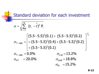
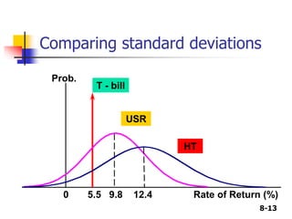
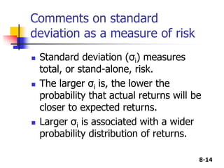
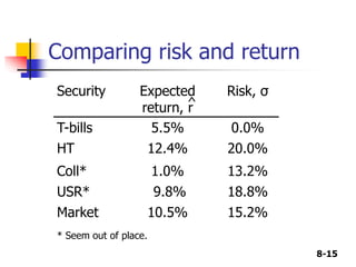
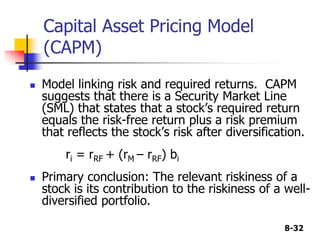
This document discusses risk and rates of return in investments. It defines key concepts like stand-alone risk, portfolio risk, standard deviation as a measure of risk, beta as a measure of market risk, and the capital asset pricing model. Standard deviation measures the total risk of an investment, while beta specifically measures non-diversifiable or systematic risk. Diversification reduces unsystematic risk by combining unrelated investments. The capital asset pricing model suggests investors should be compensated only for bearing systematic risk with the market.


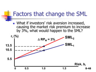


![Topic 4[1] finance](https://cdn.slidesharecdn.com/ss_thumbnails/topic41-131107182635-phpapp02-thumbnail.jpg?width=640&height=640&fit=bounds)