The document is a comprehensive review of probability calculus by Andreas Scheidegger, covering various types of random variables, their distributions, and properties such as mean, variance, and mode. It also discusses joint and conditional distributions, Bayes’ theorem, and the central limit theorem, along with applications in statistics. The review aims to provide insights into the mathematical foundations and implementations of probability within the context of random processes.

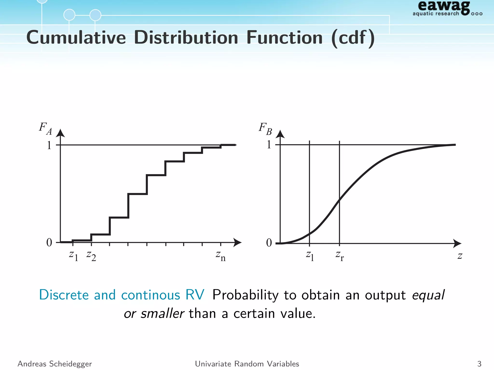
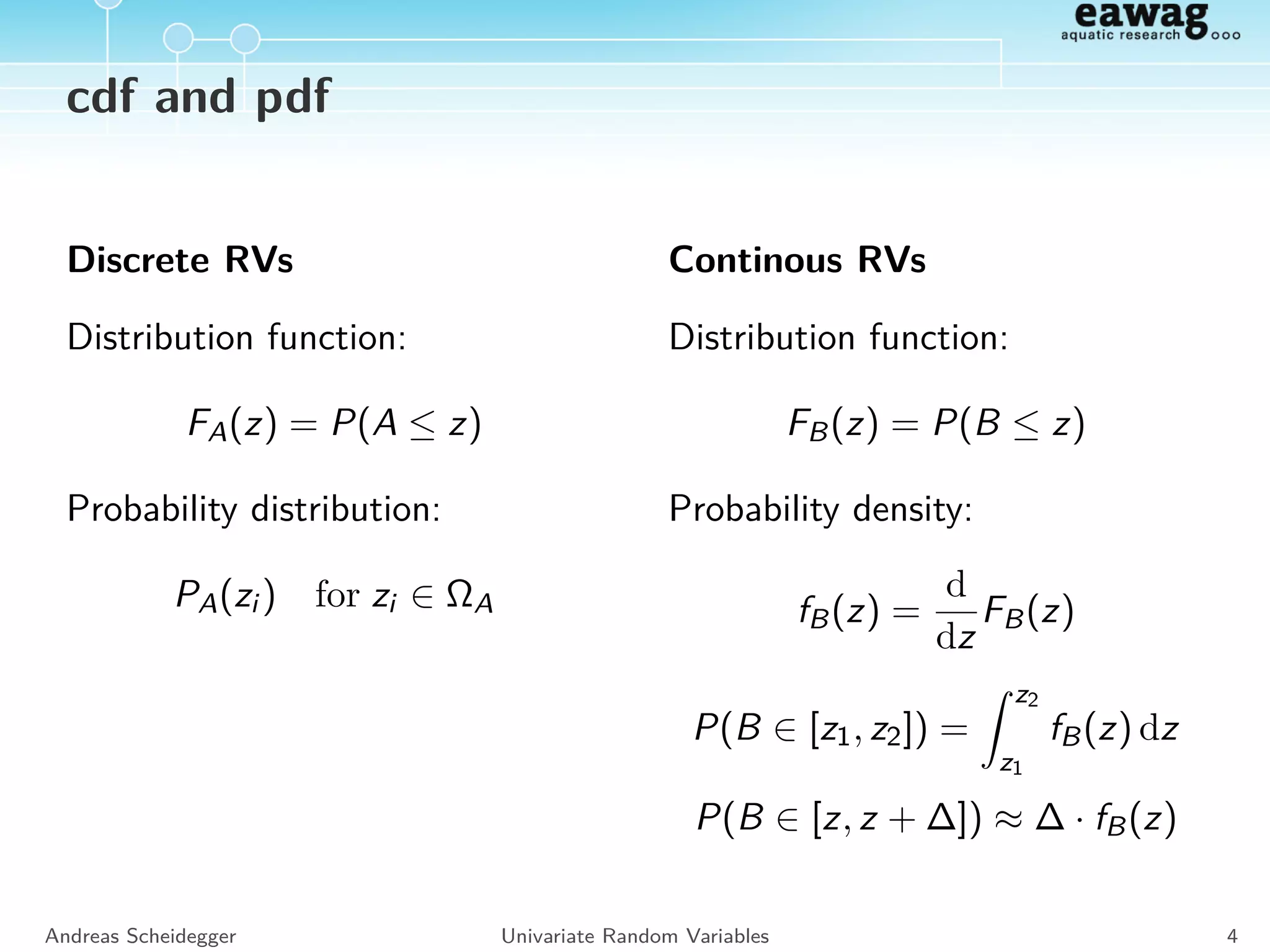
![cdf and pdf
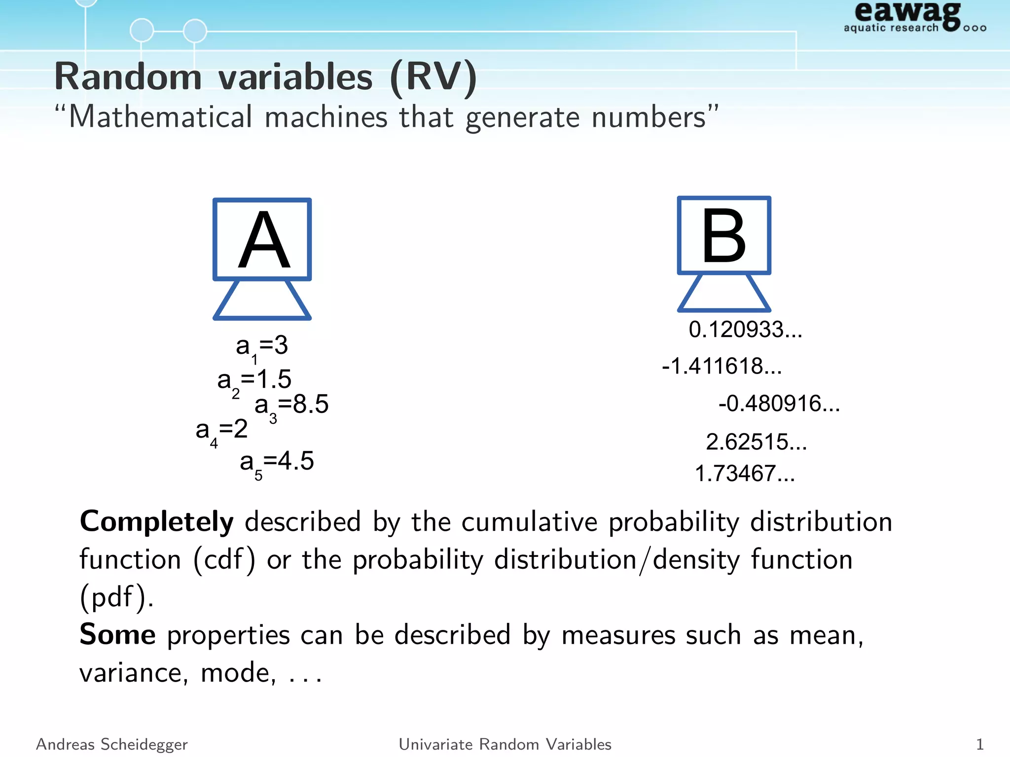
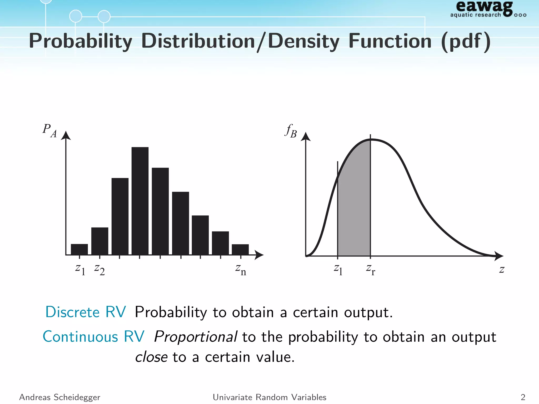
Discrete RVs
Distribution function:
FA(z) = P(A ≤ z)
Probability distribution:
PA(zi ) for zi ∈ ΩA
Continous RVs
Distribution function:
FB(z) = P(B ≤ z)
Probability density:
fB(z) =
d
dz
FB(z)
P(B ∈ [z1, z2]) =
z2
z1
fB(z) dz
P(B ∈ [z, z + ∆]) ≈ ∆ · fB(z)
Andreas Scheidegger Univariate Random Variables 4](https://image.slidesharecdn.com/probintro-170615091838/75/Review-of-probability-calculus-6-2048.jpg)
![Characteristics of Random Variables
Measures of Location
Expected value:
E[A] =
z∈ΩA
z PA(z) , E[B] =
ΩB
z fB(z) dz
Median:
Med[Z] : P(Z ≤ Med[Z]) = P(Z Med[Z]) = Q0.5[Z]
Quantiles:
Qp[Z] : P(Z ≤ Qp[Z]) = p and P(Z Qp[Z]) = 1 − p
Mode:
Mode[A] = arg max
zi ∈ΩA
PA(zi ) , Mode[B] = arg max
z∈ΩB
fB(z)
Andreas Scheidegger Univariate Random Variables 5](https://image.slidesharecdn.com/probintro-170615091838/75/Review-of-probability-calculus-7-2048.jpg)
![Characteristics of Random Variables
Measures of Location
Expected value of a function of a RV:
E[g(A)] =
z∈ΩA
g(z)PA(z)
E[g(B)] =
ΩB
g(z)fB(z) dz
Andreas Scheidegger Univariate Random Variables 6](https://image.slidesharecdn.com/probintro-170615091838/75/Review-of-probability-calculus-8-2048.jpg)
![Characteristics of Random Variables
Measures of Location
Expected value of a function of a RV:
E[g(A)] =
z∈ΩA
g(z)PA(z)
E[g(B)] =
ΩB
g(z)fB(z) dz
Attention!
E[g(X)] = g (E[X])
Andreas Scheidegger Univariate Random Variables 6](https://image.slidesharecdn.com/probintro-170615091838/75/Review-of-probability-calculus-9-2048.jpg)
![Characteristics of Random Variables
Measures of Extension
Variance:
Var[Z] = E Z − E[Z]
2
Standard Deviation:
SD[Z] = Var[Z]
Inter-Quantile Range:
QRp[Z] = Q(1+p)/2[Z] − Q(1−p)/2[Z]
Andreas Scheidegger Univariate Random Variables 7](https://image.slidesharecdn.com/probintro-170615091838/75/Review-of-probability-calculus-10-2048.jpg)
![Characteristics of Random Variables
E[aZ + b] = a E[Z] + b
E[Z1 ± Z2] = E[Z1] ± E[Z2]
Var[Z] = E[Z2
] − E[Z]2
Var[aZ + b] = a2
Var[Z]
Only if Z1 and Z2 are independent:
Var[Z1 ± Z2] = Var[Z1] + Var[Z2]
Andreas Scheidegger Univariate Random Variables 8](https://image.slidesharecdn.com/probintro-170615091838/75/Review-of-probability-calculus-11-2048.jpg)
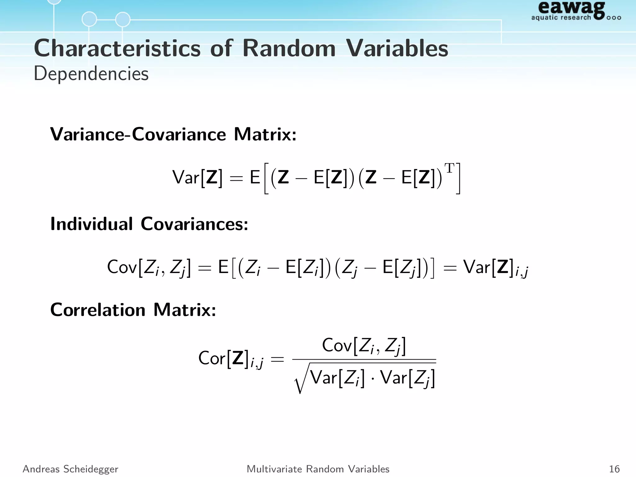
![Characteristics of Random Variables
Dependencies
Variance-Covariance Matrix:
Var[Z] = E Z − E[Z] Z − E[Z]
T
Individual Covariances:
Cov[Zi , Zj] = E Zi − E[Zi ] Zj − E[Zj] = Var[Z]i,j
Correlation Matrix:
Cor[Z]i,j =
Cov[Zi , Zj]
Var[Zi ] · Var[Zj]
Andreas Scheidegger Multivariate Random Variables 16](https://image.slidesharecdn.com/probintro-170615091838/75/Review-of-probability-calculus-22-2048.jpg)
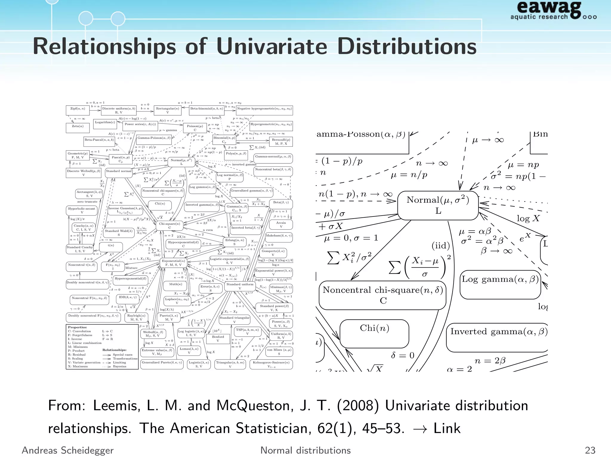
![Relationships of Univariate Distributions
Figure 1. Univariate distribution relationships.
The American Statistician, February 2008, Vol. 62, No. 1 47
Downloadedby[Lib4RI]at02:2428May2013
at02:2428May2013
From: Leemis, L. M. and McQueston, J. T. (2008) Univariate distribution
relationships. The American Statistician, 62(1), 45–53. → Link
Andreas Scheidegger Normal distributions 23](https://image.slidesharecdn.com/probintro-170615091838/75/Review-of-probability-calculus-31-2048.jpg)