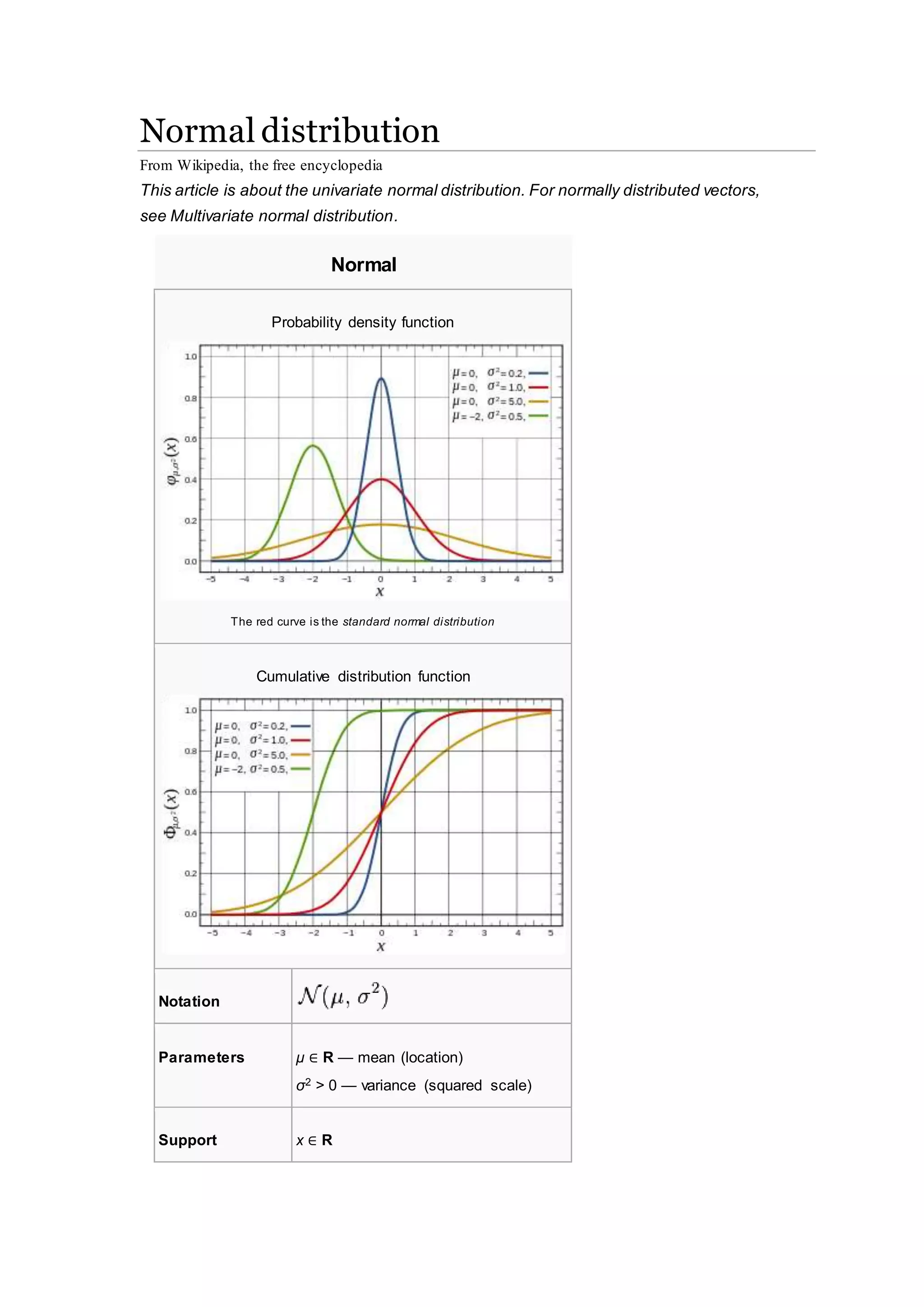
The document discusses the normal distribution, also called the Gaussian distribution, which is a very commonly used probability distribution in statistics. It has two parameters: the mean μ, which is the expected value, and the standard deviation σ. The normal distribution is symmetric around the mean and bell-shaped. It is useful because of the central limit theorem and is applied when variables are expected to be the sum of many independent processes.
Statistik 1 6 distribusi probabilitas normalSelvin Hadi
This document discusses the key characteristics and concepts of the normal probability distribution. It outlines six goals related to understanding the normal distribution, its properties, calculating z-values, and using the normal distribution to approximate the binomial probability distribution. The key points covered include defining the mean, standard deviation, and shape of the normal curve; transforming variables to the standard normal distribution; and determining probabilities based on the areas under the normal curve.
Chap05 continuous random variables and probability distributionsJudianto Nugroho
This chapter discusses continuous random variables and probability distributions, including the normal distribution. It introduces continuous random variables and their probability density functions. It describes the key characteristics and properties of the uniform and normal distributions. It also discusses how to calculate probabilities using the normal distribution, including how to standardize a normal distribution and use normal distribution tables.
This document provides an overview of the normal distribution including:
- Its bell-shaped, symmetric nature with the mean, median, and mode being equal
- That it has a single peak at the center and the area under the curve is equal to 100%
- The empirical rule stating that about 68%, 95%, and 99.7% of values lie within 1, 2, and 3 standard deviations of the mean respectively
- How to calculate z-scores using the formula z = (x - μ) / σ and look them up on a z-table
- Several examples of calculating z-scores and finding values given the mean and standard deviation
The document discusses sampling distributions and summarizes key points about the sampling distribution of the mean for both known and unknown population variance. It states that the sampling distribution of the mean has a normal distribution with mean equal to the population mean and variance equal to the population variance divided by the sample size when the population variance is known. When the population variance is unknown, the sampling distribution follows a t-distribution if the population is normally distributed.
4 2 continuous probability distributionnLama K Banna
Here are the steps to solve this problem:
a) Find the z-score corresponding to 115 mm Hg: (115 - 85)/13 = 2.31
The proportion that is NOT severely hypertensive is 1 - P(Z >= 2.31) = 1 - 0.0103 = 0.9897
b) Find the z-score corresponding to 90 mm Hg: (90 - 85)/13 = 0.3846
The proportion that will be asked to consult a physician is P(Z >= 0.3846) = 0.6507
c) Find the z-scores corresponding to the mildly hypertensive range:
(90 - 85)/13 = 0.3846
(
The document discusses the normal probability distribution and related concepts. It defines continuous random variables and probability density functions, and describes how the normal distribution is characterized by its mean and standard deviation. It also explains how to standardize a normal random variable to the standard normal distribution in order to use normal probability tables and find probabilities of intervals. Key steps covered include transforming values to z-scores and looking up the corresponding areas in the standard normal distribution table.
This document contains a chapter from a statistics textbook on the normal probability distribution. It includes objectives, examples, and explanations of key concepts regarding the normal distribution, such as:
- The properties of the normal distribution curve including that it is symmetric and bell-shaped.
- How to standardize a normal random variable and find areas under the standard normal curve using z-scores and tables of normal probabilities.
- Interpreting the area under the normal curve as probabilities or proportions for real-world examples like IQ scores and weights of animals.
The document discusses properties of normal distributions and the standard normal distribution. It provides examples of finding probabilities and values associated with normal distributions. The key points are:
- Normal distributions are continuous and bell-shaped. The mean, median and mode are equal.
- The standard normal distribution has a mean of 0 and standard deviation of 1.
- Probabilities under the normal curve can be found using z-scores and the standard normal table.
- Values like z-scores can be determined by finding the corresponding cumulative area in the standard normal table.
The document discusses the normal distribution and its key properties. It introduces the normal probability density function and how it is characterized by a mean and variance. Some key properties covered are that the sum of independent normally distributed variables is also normally distributed, with the mean being the sum of the individual means and the variance being the sum of the individual variances. It also discusses how to compute probabilities and find values for the standard normal distribution.
Bba 3274 qm week 3 probability distributionStephen Ong
This document provides an introduction and overview of probability distributions. It begins by defining random variables and explaining the difference between discrete and continuous random variables. It then discusses several common probability distributions including the binomial, normal, F, exponential, and Poisson distributions. For each distribution, it provides the key formulas and explains how to calculate values such as the expected value and variance. It also demonstrates how to use Excel functions to calculate probabilities and other measures for these distributions. The document aims to help students understand different probability distributions and how to apply them to calculate relevant metrics.
CABT SHS Statistics & Probability - The Standard Normal DistributionGilbert Joseph Abueg
This document provides an overview of the normal distribution and how to calculate probabilities and areas under the standard normal curve. It discusses the key properties of the normal distribution including that it is symmetric and bell-shaped. It also presents the process for finding areas in different regions of the standard normal distribution, including tails, between values with the same sign, between values with opposite signs, and cumulative areas. Examples are provided for calculating areas in each of these four cases. The document is intended as a lecture presentation for a Grade 11 statistics and probability class to teach students how to work with the normal distribution and standard normal curve.
PG STAT 531 Lecture 3 Graphical and Diagrammatic Representation of DataAashish Patel
The document discusses various methods of graphically and diagrammatically representing statistical data, including:
1) Bar diagrams, pie charts, and line graphs that use bars, circles, or lines to show relationships between data points;
2) Histograms that use rectangles to show frequency distributions; and
3) Frequency polygons and curves that smooth data points to reveal trends, and ogives that show cumulative frequencies. Graphical representations make trends and relationships easier for experts and non-experts to understand versus numerical representations alone.
Here are the solutions to the exercises:
1. The area under the standard normal curve between z=-∞ and z=2 is 0.9772 (using the standard normal table)
2. The probability that a z value will be between -2.55 and +2.55 is 0.9932 (using the standard normal table)
3. The proportion of z values between -2.74 and 1.53 is 0.9950
4. P(z ≥ 2.71) = 1 - 0.9958 = 0.0042
5. P(.84 ≤ z ≤ 2.45) = 0.8036 - 0.1967 = 0.6069
This chapter discusses methods for constructing confidence intervals for differences between population means and proportions in various sampling situations. It covers confidence intervals for the difference between two dependent or paired sample means, two independent sample means when population variances are known or unknown, and two independent population proportions. It also addresses determining required sample sizes to estimate a mean or proportion within a specified margin of error.
The document introduces the Gaussian or normal distribution, its key properties, and how it can be used for inference. The Gaussian distribution is symmetrical and bell-shaped. It is completely defined by its mean and standard deviation. By transforming data into z-scores, the standard normal distribution can be applied to understand the probabilities of outcomes in any normal distribution. The Gaussian distribution and z-scores allow researchers to assess likelihoods and make inferences about variable values based on their known distribution.
A random variable is a variable whose values are determined by the outcome of a random experiment and can be used to model probabilities. Examples of random variables include the sum of dice rolls or number of heads from coin tosses. A probability distribution assigns probabilities to each possible value of a random variable. It must satisfy the properties that probabilities are greater than or equal to 0 and sum to 1. Common probability distributions include the binomial and normal distributions.
Quantitative Methods for Management_MBA_Bharathiar University probability dis...Victor Seelan
unit 3 probability distribution
Probability – definitions – addition and multiplication Rules (only statements) – simple business application problems – probability distribution – expected value concept – theoretical probability distributions – Binomial, Poison and Normal – Simple problems applied to business.
This document discusses three probability distributions: the binomial, Poisson, and normal distributions. It provides details on the Poisson distribution, including its definition as a model for independent and random events with a constant probability over time. Examples are given of how the Poisson distribution can model the number of occurrences in a fixed time period, such as telephone calls in an hour. The key properties of the Poisson distribution are that the mean and variance are equal to the parameter lambda.
This document discusses sampling distributions and their properties. It provides steps to construct a sampling distribution of sample means from a population. Specifically, it shows how to determine the number of possible samples, calculate the mean of each sample, and compile these into a frequency distribution. The sampling distribution's mean equals the population mean, while its variance is the population variance divided by the sample size. Examples demonstrate calculating the mean and variance of sampling distributions for different sample sizes. Key properties of sampling distributions are summarized.
A random variable is a rule that assigns a numerical value to each outcome of an experiment. Random variables can be either discrete or continuous. A discrete random variable may assume countable values, while a continuous random variable can assume any value in an interval. The probability distribution of a random variable describes the probabilities of the variable assuming different values. For a continuous random variable, the probability of it assuming a value within an interval is given by the area under the probability density function within that interval.
The document provides an outline and explanation of key concepts related to the normal distribution. It begins with an introduction to probability distributions for continuous random variables and the definition of a density curve. It then defines terms and symbols used in the normal distribution, including mean, standard deviation, and z-scores. The document explains the characteristics of the normal distribution graphically and provides examples of finding areas under the normal curve using z-tables. It concludes with examples of finding unknown z-values and calculating probabilities for specific scenarios involving the normal distribution.
The document discusses the normal distribution and its key properties: bell-shaped and symmetrical around the mean, extending from negative to positive infinity with an area under the curve of 1. Approximately 95% and 99.9% of the distribution lies within 2 and 3 standard deviations of the mean, respectively. It also discusses how to calculate probabilities using the standard normal distribution where the mean is 0 and standard deviation is 1, and how to standardize other normal distributions.
Normal distribution and sampling distributionMridul Arora
This document provides an overview of Chapter 5 from the textbook, which covers normal probability distributions. Section 5.1 introduces normal distributions and the standard normal distribution, including their key properties and how to interpret related graphs. It describes how any normal distribution can be transformed into a standard normal distribution for calculation purposes. Section 5.1 also shows how to find areas under the standard normal curve using the standard normal table. Section 5.2 discusses how to calculate probabilities for normally distributed variables by relating them to areas under the normal curve. It provides examples of finding probabilities and expected values.
Demonstration of a z transformation of a normal distributionkkong
The document demonstrates how to transform a normal distribution with a mean of 10 and standard deviation of 2 into a standard normal distribution with a mean of 0 and standard deviation of 1 using the z-transformation formula. It shows that the z-transformation shifts and compresses the original distribution allowing its probabilities to be determined using standard normal distribution tables. As an example, it finds the probability of a value less than or equal to 8 in the original distribution to be 15.9% by transforming it to the equivalent value of -1 in the standard normal distribution.
This document provides an overview of Chapter 4 from the textbook "Discrete Probability Distributions" by Larson/Farber. The chapter outlines key concepts related to discrete probability distributions including distinguishing between discrete and continuous random variables, constructing probability distributions, and calculating mean, variance, standard deviation, and expected value. It also previews the topics to be covered in Sections 4.1 on probability distributions and 4.2 on binomial distributions.
1. Continuous random variables are defined over intervals rather than discrete points. The probability that a continuous random variable takes on a value in an interval from a to b is given by an integral of the probability density function f(x) over that interval.
2. The probability density function f(x) defines the probabilities of intervals of the continuous random variable rather than individual points. It has the properties that it is always nonnegative and its integral over all x is 1.
3. The cumulative distribution function F(x) gives the probability that the random variable takes on a value less than or equal to x. It is defined as the integral of the probability density function from negative infinity to x.
1. The central limit theorem states that the distribution of sample means approaches a normal distribution as sample size increases, even if the population is not normally distributed.
2. For a sample size of 30 or more, the distribution of sample means can be approximated as a normal distribution, allowing probabilities to be found using the normal distribution.
3. The mean of the distribution of sample means is the same as the population mean, and its standard deviation is the population standard deviation divided by the square root of the sample size.
The normal distribution, also called the Gaussian distribution, is a very common continuous probability distribution. It is often used to represent real-valued random variables whose actual distributions are unknown. The normal distribution depends on two parameters: the mean (μ) and the variance (σ2). It is symmetric and bell-shaped, with the mean, median and mode all being equal and located at the center. Some key properties include that approximately 68%, 95% and 99.7% of the data lies within 1, 2 and 3 standard deviations of the mean, respectively. The normal distribution was discovered independently by de Moivre and Laplace and is also associated with Gauss.
The normal distribution, also called the Gaussian distribution, is a very common continuous probability distribution. It is often used to represent real-valued random variables whose actual distributions are unknown. The normal distribution depends on two parameters: the mean (μ) and standard deviation (σ). A random variable that follows a normal distribution is said to be normally distributed. The normal distribution is symmetric and bell-shaped. It is important in statistics and is commonly used in sciences to model natural phenomena.
The document discusses the standard normal distribution. It defines the standard normal distribution as having a mean of 0, a standard deviation of 1, and a bell-shaped curve. It provides examples of how to find probabilities and z-scores using the standard normal distribution table or calculator. For example, it shows how to find the probability of an event being below or above a given z-score, or between two z-scores. It also shows how to find the z-score corresponding to a given cumulative probability.
The Gaussian distribution, also known as the normal distribution, is a continuous probability distribution with a bell-shaped curve. It is defined by two parameters: the mean and the standard deviation. The normal distribution is symmetric about its mean and has many useful properties, including that the sum of independent normal variables is also normally distributed. It is one of the most important probability distributions in statistics.
The document provides information about several theoretical probability distributions including the normal, t, and chi-square distributions. It discusses key properties such as the mean, standard deviation, and shape of the normal distribution curve. Examples are given to demonstrate how to calculate areas under the normal distribution curve and find z-scores. The t-distribution is introduced as similar to the normal but used for smaller sample sizes. The chi-square distribution is defined as used for hypothesis testing involving categorical data.
1. The standard deviation is a measure of how spread out numbers are from the average value.
2. It is calculated by taking the square root of the variance, which is the average of the squared differences from the mean.
3. When only a sample of data is available rather than the entire population, the sample standard deviation is estimated using N-1 in the denominator rather than N to reduce bias, though some bias still remains for small samples.
ders 3.2 Unit root testing section 2 .pptxErgin Akalpler
The document provides information about several theoretical probability distributions including the normal, t, and chi-square distributions. It discusses their key properties and formulas. For the normal distribution, it covers the empirical rule, skewness, kurtosis, and how to calculate z-scores. Examples are given for finding areas under the normal curve and performing hypothesis tests using the t and chi-square distributions.
This document discusses continuous probability distributions, including the normal and exponential distributions. It defines a continuous random variable and probability density function. The key properties of the normal distribution are described, such as its bell-shaped, symmetric curve defined by the mean and standard deviation. Examples demonstrate how to generate random normal variables and calculate probabilities using R commands. The exponential distribution is also introduced, which has a positively skewed density curve where the mean and standard deviation are equal.
The document discusses the normal distribution, which produces a symmetrical bell-shaped curve. It has two key parameters - the mean and standard deviation. According to the empirical rule, about 68% of values in a normal distribution fall within one standard deviation of the mean, 95% within two standard deviations, and 99.7% within three standard deviations. The normal distribution is commonly used to model naturally occurring phenomena that tend to cluster around an average value, such as heights or test scores.
The PPT covered the distinguish between discrete and continuous distribution. Detailed explanation of the types of discrete distributions such as binomial distribution, Poisson distribution & Hyper-geometric distribution.
This document discusses higher order moments, variance, and standard deviation of random variables. It defines higher order moments as moments beyond the 4th moment, and explains that they can be used to describe further shape parameters beyond variance, skewness, and kurtosis. The document also defines variance as a measure of how spread out a random variable's distribution is, and standard deviation as the square root of variance. It provides formulas for calculating variance and standard deviation of both discrete and continuous random variables. Several examples are worked through to demonstrate calculating variance for different probability distributions.
Chapter 2 normal distribution grade 11 pptRandyNarvaez
This chapter introduces the normal probability distribution, which is an important distribution in statistics. The normal distribution is bell-shaped and symmetric around the mean. Examples of data that follow a normal distribution include physical characteristics like height or weight, as well as test scores and natural phenomena like river water volumes. Key properties of the normal distribution are discussed, including that the mean equals the median and mode, and the spread is determined by the standard deviation. Formulas for the normal probability distribution function are provided.
Normal Distribution – Introduction and PropertiesSundar B N
In this video you can see Normal Distribution – Introduction and Properties.
Watch the video on above ppt
https://www.youtube.com/watch?v=ocTXHLWsec8&list=PLBWPV_4DjPFO6RjpbyYXSaZHiakMaeM9D&index=4
Subscribe to Vision Academy
https://www.youtube.com/channel/UCjzpit_cXjdnzER_165mIiw
The document discusses the normal distribution and some of its key properties. It also discusses the central limit theorem and how the distribution of sample means approaches a normal distribution as the sample size increases. Additionally, it covers how to transform a normally distributed variable into a standard normal variable using z-scores and how the normal distribution can be used to approximate the binomial distribution through a correction for continuity.
This document discusses sampling distributions and how to calculate confidence intervals for statistical parameters like the mean and variance of a population based on a sample. It describes key distributions like the normal, chi-square and Student's t distribution. It provides the formulas to determine confidence intervals for the mean when the population variance is known or unknown, and for the variance. The confidence intervals indicate the range within which the true parameter is likely to fall, given a sample estimate and a confidence level like 95%.
Please Subscribe to this Channel for more solutions and lectures
http://www.youtube.com/onlineteaching
Chapter 6: Normal Probability Distribution
6.1: The Standard Normal Distribution
lesson 3.1 Unit root testing section 1 .pptxErgin Akalpler
The document discusses key concepts related to the normal distribution, including its properties, formula, and uses. Some key points:
- The normal distribution is a bell-shaped curve that is symmetric around the mean. Many natural phenomena approximate it.
- It is defined by two parameters: the mean and standard deviation. Approximately 68% of values fall within one standard deviation of the mean, 95% within two standard deviations, and 99.7% within three standard deviations.
- The normal distribution follows a specific formula involving the mean, standard deviation, and z-scores.
- Other concepts discussed include skewness, kurtosis, the t-distribution and how it resembles the normal distribution, and
How to Setup Default Value for a Field in Odoo 17Celine George
In Odoo, we can set a default value for a field during the creation of a record for a model. We have many methods in odoo for setting a default value to the field.
A Visual Guide to 1 Samuel | A Tale of Two HeartsSteve Thomason
These slides walk through the story of 1 Samuel. Samuel is the last judge of Israel. The people reject God and want a king. Saul is anointed as the first king, but he is not a good king. David, the shepherd boy is anointed and Saul is envious of him. David shows honor while Saul continues to self destruct.
Elevate Your Nonprofit's Online Presence_ A Guide to Effective SEO Strategies...TechSoup
Whether you're new to SEO or looking to refine your existing strategies, this webinar will provide you with actionable insights and practical tips to elevate your nonprofit's online presence.
How to Manage Reception Report in Odoo 17Celine George
A business may deal with both sales and purchases occasionally. They buy things from vendors and then sell them to their customers. Such dealings can be confusing at times. Because multiple clients may inquire about the same product at the same time, after purchasing those products, customers must be assigned to them. Odoo has a tool called Reception Report that can be used to complete this assignment. By enabling this, a reception report comes automatically after confirming a receipt, from which we can assign products to orders.
Andreas Schleicher presents PISA 2022 Volume III - Creative Thinking - 18 Jun...EduSkills OECD
Andreas Schleicher, Director of Education and Skills at the OECD presents at the launch of PISA 2022 Volume III - Creative Minds, Creative Schools on 18 June 2024.
Level 3 NCEA - NZ: A Nation In the Making 1872 - 1900 SML.pptHenry Hollis
The History of NZ 1870-1900.
Making of a Nation.
From the NZ Wars to Liberals,
Richard Seddon, George Grey,
Social Laboratory, New Zealand,
Confiscations, Kotahitanga, Kingitanga, Parliament, Suffrage, Repudiation, Economic Change, Agriculture, Gold Mining, Timber, Flax, Sheep, Dairying,
Gender and Mental Health - Counselling and Family Therapy Applications and In...PsychoTech Services
A proprietary approach developed by bringing together the best of learning theories from Psychology, design principles from the world of visualization, and pedagogical methods from over a decade of training experience, that enables you to: Learn better, faster!
Gender and Mental Health - Counselling and Family Therapy Applications and In...
Normal distribution
1. Normal distribution
From Wikipedia, the free encyclopedia
This article is about the univariate normal distribution. For normally distributed vectors,
see Multivariate normal distribution.
Normal
Probability density function
The red curve is the standard normal distribution
Cumulative distribution function
Notation
Parameters μ ∈ R — mean (location)
σ2 > 0 — variance (squared scale)
Support x ∈ R
2. pdf
CDF
Quantile
Mean μ
Median μ
Mode μ
Variance
Skewness 0
Ex. kurtosis 0
Entropy
MGF
CF
Fisher
information
In probability theory, the normal (or Gaussian) distribution is a very commonly
occurring continuous probability distribution—a function that tells the probability that any real
observation will fall between any two real limits or real numbers, as the curve approaches
zero on either side. Normal distributions are extremely important in statistics and are often
used in the natural and social sciences for real-valued random variables whose distributions
are not known.
3. The normal distribution is immensely useful because of the central limit theorem, which
states that, under mild conditions, the mean of many random variables independently drawn
from the same distribution is distributed approximately normally, irrespective of the form of
the original distribution: physical quantities that are expected to be the sum of many
independent processes (such as measurement errors) often have a distribution very close to
the normal. Moreover, many results and methods (such as propagation of
uncertainty and least squares parameter fitting) can be derived analytically in explicit form
when the relevant variables are normally distributed.
The Gaussian distribution is sometimes informally called the bell curve. However, many
other distributions are bell-shaped (such as Cauchy's, Student's, and logistic). The
terms Gaussian function and Gaussian bell curve are also ambiguous because they
sometimes refer to multiples of the normal distribution that cannot be directly interpreted in
terms of probabilities.
A normal distribution is
The parameter μ in this definition is the mean or expectation of the distribution (and also
its median and mode). The parameter σis its standard deviation; its variance is
therefore σ 2. A random variable with a Gaussian distribution is said to be normally
distributed and is called a normal deviate.
If μ = 0 and σ = 1, the distribution is called the standard normal distribution or the unit
normal distribution, and a random variable with that distribution is a standard normal
deviate.
The normal distribution is the only absolutely continuousdistribution all of
whose cumulants beyond the first two (i.e., other than the mean and variance) are zero.
It is also the continuous distribution with the maximum entropy for a given mean and
variance.[3][4]
The normal distribution is a subclass of the elliptical distributions. The normal distribution
is symmetric about its mean, and is non-zero over the entire real line. As such it may not
be a suitable model for variables that are inherently positive or strongly skewed, such as
the weight of a person or the price of a share. Such variables may be better described by
other distributions, such as the log-normal distribution or the Pareto distribution.
The value of the normal distribution is practically zero when the value x lies more than a
few standard deviations away from the mean. Therefore, it may not be an appropriate
model when one expects a significant fraction of outliers—values that lie many standard
deviations away from the mean — and least squares and other statistical
inference methods that are optimal for normally distributed variables often become highly
4. unreliable when applied to such data. In those cases, a more heavy-tailed distribution
should be assumed and the appropriate robust statistical inference methods applied.
The Gaussian distribution belongs to the family of stable distributions which are the
attractors of sums of independent, identically distributed distributions whether or not the
mean or variance is finite. Except for the Gaussian which is a limiting case, all stable
distributions have heavy tails and infinite variance.
Contents
[hide]
1 Definition
o 1.1 Standard normal distribution
o 1.2 General normal distribution
o 1.3 Notation
o 1.4 Alternative parameterizations
2 Properties
o 2.1 Symmetries and derivatives
o 2.2 Moments
o 2.3 Fourier transform and characteristic function
o 2.4 Moment and cumulant generating functions
3 Cumulative distribution function
o 3.1 Standard deviation and tolerance intervals
o 3.2 Quantile function
4 Zero-variance limit
5 The central limit theorem
6 Operations on normal deviates
o 6.1 Infinite divisibility and Cramér's theorem
o 6.2 Bernstein's theorem
7 Other properties
8 Related distributions
o 8.1 Operations on a single random variable
o 8.2 Combination of two independent random variables
o 8.3 Combination of two or more independent random variables
o 8.4 Operations on the density function
o 8.5 Extensions
9 Normality tests
10 Estimation of parameters
11 Bayesian analysis of the normal distribution
o 11.1 The sum of two quadratics
11.1.1 Scalar form
11.1.2 Vector form
o 11.2 The sum of differences from the mean
o 11.3 With known variance
o 11.4 With known mean
o 11.5 With unknown mean and unknown variance
12 Occurrence
o 12.1 Exact normality
o 12.2 Approximate normality
o 12.3 Assumed normality
o 12.4 Produced normality
13 Generating values from normal distribution
5. 14 Numerical approximations for the normal CDF
15 History
o 15.1 Development
o 15.2 Naming
16 See also
17 Notes
18 Citations
19 References
20 External links
Definition[edit]
Standard normal distribution[edit]
The simplest case of a normal distribution is known as the standard normal distribution.
This is a special case where μ=0 and σ=1, and it is described by this probability density
function:
The factor in this expression ensures that the total area under the curve ϕ(x)
is equal to one.[5] The 1/2 in the exponent ensures that the distribution has unit
variance (and therefore also unit standard deviation). This function is symmetric
around x=0, where it attains its maximum value ; and has inflection
points at +1 and −1.
Authors may differ also on which normal distribution should be called the "standard"
one. Gauss himself defined the standard normal as having variance σ2 = 1/2, that is
Stigler[6] goes even further, defining the standard normal with variance σ2 = 1/2π :
General normal distribution[edit]
Any normal distribution is a version of the standard normal distribution
whose domain has been stretched by a factor σ (the standard deviation) and
then translated by μ (the mean value):
The probability density must be scaled by so that the integral is
still 1.
If Z is a standard normal deviate, then X = Zσ + μ will have a normal
distribution with expected value μ and standard deviation σ. Conversely,
6. if X is a general normal deviate, then Z = (X − μ)/σ will have a standard
normal distribution.
Every normal distribution is the exponential of a quadratic function:
where a is negative and c is . In this
form, the mean value μ is −b/(2a), and the variance σ2 is −1/(2a).
For the standard normal distribution, a is −1/2, b is zero,
and c is .
Notation[edit]
The standard Gaussian distribution (with zero mean and unit
variance) is often denoted with the Greek letter ϕ (phi).[7] The
alternative form of the Greek phi letter, φ, is also used quite often.
The normal distribution is also often denoted by N(μ, σ2).[8] Thus
when a random variable X is distributed normally with mean μ and
variance σ2, we write
Alternative parameterizations[edit]
Some authors advocate using the precision τ as the parameter
defining the width of the distribution, instead of the deviationσ or
the variance σ2. The precision is normally defined as the
reciprocal of the variance, 1/σ2.[9] The formula for the distribution
then becomes
This choice is claimed to have advantages in numerical
computations when σ is very close to zero and simplify
formulas in some contexts, such as in the Bayesian
inference of variables with multivariate normal distribution.
Occasionally, the precision τ is 1/σ, the reciprocal of the
standard deviation; so that
According to Stigler, this formulation is advantageous
because of a much simpler and easier-to-remember
formula, the fact that the pdf has unit height at zero, and
7. simple approximate formulas for the quantiles of the
distribution.
Properties[edit]
Symmetries and derivatives[edit]
The normal distribution f(x), with any mean μ and any
positive deviation σ, has the following properties:
It is symmetric around the point x = μ, which is at
the same time the mode, the median and the mean
of the distribution.[10]
It is unimodal: its first derivative is positive for x < μ,
negative for x > μ, and zero only at x = μ.
Its density has two inflection points (where the
second derivative of f is zero and changes sign),
located one standard deviation away from the
mean, namely at x = μ − σ and x = μ + σ.[10]
Its density is log-concave.[10]
Its density is infinitely differentiable,
indeed supersmooth of order 2.[11]
Its second derivative f′′(x) is equal to its derivative
with respect to its variance σ2
Furthermore, the density ϕ of the standard normal
distribution (with μ = 0 and σ = 1) also has the following
properties:
Its first derivative ϕ′(x) is −xϕ(x).
Its second derivative ϕ′′(x) is (x2 − 1)ϕ(x)
More generally, its n-th derivative ϕ(n)(x) is
(−1)nHn(x)ϕ(x), where Hn is the Hermite
polynomial of order n.[12]
It satisfies the differential equation
or
Moments[edit]
See also: List of integrals of Gaussian
functions
8. The plain and absolute moments of a
variable X are the expected values
of Xp and |X|p,respectively. If the expected
value μof X is zero, these parameters are
called central moments. Usually we are
interested only in moments with integer
order p.
If X has a normal distribution, these
moments exist and are finite for
any p whose real part is greater than −1.
For any non-negative integer p, the plain
central moments are
Here n!! denotes the double factorial,
that is, the product of every number
from n to 1 that has the same parity
as n.
The central absolute moments coincide
with plain moments for all even orders,
but are nonzero for odd orders. For any
non-negative integer p,
The last formula is valid also for
any non-integer p > −1. When the
mean μ is not zero, the plain and
absolute moments can be
expressed in terms of confluent
hypergeometric
functions 1F1 and U.[citation needed]
9. These expressions remain
valid even if p is not
integer. See
also generalized Hermite
polynomials.
Order Non-central moment Central moment
1 μ 0
2 μ2
+ σ2
σ 2
3 μ3
+ 3μσ2
0
4 μ4
+ 6μ2
σ2
+ 3σ4
3σ 4
5 μ5
+ 10μ3
σ2
+ 15μσ4
0
6 μ6
+ 15μ4
σ2
+ 45μ2
σ4
+ 15σ6
15σ 6
7 μ7
+ 21μ5
σ2
+ 105μ3
σ4
+ 105μσ6
0
8 μ8
+ 28μ6
σ2
+ 210μ4
σ4
+ 420μ2
σ6
+ 105σ8
105σ 8
Fourier transform
and characteristic
function[edit]
The Fourier transform of a
normal distribution f with
mean μ and
deviation σ is[13]
where i is
the imaginary unit. If
the mean μ is zero, the
10. first factor is 1, and the
Fourier transform is
also a normal
distribution on
the frequency domain,
with mean 0 and
standard deviation 1/σ.
In particular, the
standard normal
distribution ϕ (with μ=0
and σ=1) is
an eigenfunction of the
Fourier transform.
In probability theory,
the Fourier transform
of the probability
distribution of a real-
valued random
variable X is called
thecharacteristic
function of that
variable, and can be
defined as
the expected
value of eitX, as a
function of the real
variable t(the frequenc
y parameter of the
Fourier transform).
This definition can be
analytically extended
to a complex-value
parameter t.[14]
Moment and
cumulant
generating
functions[edit]
The moment
generating function of
a real random
variable X is the
11. expected value of etX,
as a function of the
real parametert. For a
normal distribution
with mean μ and
deviation σ, the
moment generating
function exists and is
equal to
The cumulant
generating
function is the
logarithm of the
moment
generating
function, namely
Since this is a
quadratic
polynomial
in t, only the
first
two cumulants
are nonzero,
namely the
mean μ and
the
variance σ2.
Cumulati
ve
distributi
on
function[
edit]
The
cumulative