Download to read offline

![3 Results
The experimental values for fo, amplitude response, and phase response (at fo) are listed in Table
1.
Table 1 – Comparison of the experimental values to the simulated values.
Experimental Simulated,
Oscilloscope
Simulated, Bode Plot
Cutoff Frequency (fo)
[Hz]
9,000 ± 400 9,000 8,800 ± 800
Amplitude Response 0.70 ± 0.02 0.708 ± 0.001 0.71 ± 0.02
Phase Response
[Degrees]
-45 ± 3 -47 ± 2 -45.0 ± 0.1
However, the frequency, amplitude response, and phase response acquired experimentally agree
with the simulated values. The Figures 2 and 3 show the experimental values of the amplitude
response H and the phase response 𝜙 plotted against frequency, in a log-log and a log-lin plot,
respectively. The areas of interest, H = 0.707 in Figure 2 and 𝜙 =-45° in Figure 3, were enlarged.
Figure 1
Figure 2 –The amplitude response for an LPF, with portion of graph from H = 10-0.1
to
H = 10-0.3
enlarged.](https://image.slidesharecdn.com/9c8438ca-6566-4c89-a7de-9402feea7fdc-160826232651/85/RC-Circuit-4-320.jpg)
![References
Matlab Amplitude Response Code
clc;
clear all;
close all;
filename = 'A3 Graphs.xlsx';
A = xlsread(filename);
x=A(:,1);
y=A(:,2);
e=A(:,3);
g=[10:10:1000000];
R=460;
C=3.844*(10^(-8));
f=2*pi*g;
w=(R*C*f).^2;
j=(1./(1+w).^(1/2));
loglog(x,y,'ob');
hold on;
loglog(g,j,'-r');
errorbar(x,y,e,'.');
legend('Experimental Values','Theoretical Values' ); %inserts legend
and labels axes
xlabel('Frequency [Hz]');
ylabel('H');
axis([100 10^6 0 1]);
fullpath_filename = 'C:UsersRossPicturesGraph';
saveas(gcf,fullpath_filename,'png')](https://image.slidesharecdn.com/9c8438ca-6566-4c89-a7de-9402feea7fdc-160826232651/85/RC-Circuit-6-320.jpg)
![Matlab Phase Response Code
clc;
clear all;
close all;
filename = 'Book2.xlsx';
A = xlsread(filename);
x=A(:,1);
y=A(:,2);
e=A(:,3);
g=[10:10:1000000];
t=[0:20/99999:20]*10^((-6));
p=(-360)*t.*g;
f=atan(2*pi*g*460*(3.88*10^(-8)));
h=f*(-180/pi);
semilogx(x,y,'ob')
hold on;
semilogx(g,h,'-r');
errorbar(x,y,e,'.');
legend('Experimental Values','Theoretical Values' );
xlabel('Frequency [Hz]');
ylabel('phi [degrees]');
axis([100 10^6 0 -90]);
fullpath_filename = 'C:UsersRossPicturesGraphd';
saveas(gcf,fullpath_filename,'png')](https://image.slidesharecdn.com/9c8438ca-6566-4c89-a7de-9402feea7fdc-160826232651/85/RC-Circuit-7-320.jpg)

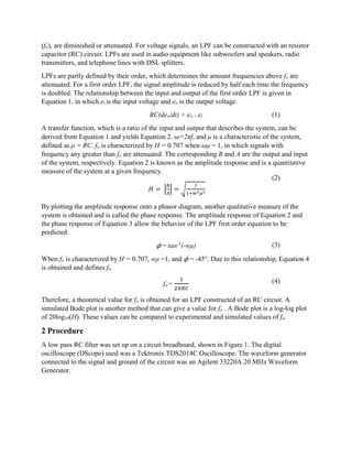
A first order low pass filter was modeled using an RC circuit with a 460 ohm resistor and 0.05 microfarad capacitor. The experimental cutoff frequency was found to be 9,000 ± 400 Hz, which matched the simulated value. The experimental amplitude response and phase response also matched theoretical values, except at 1 MHz where discrepancies occurred likely due to limitations of the waveform generator and modeling assumptions at high frequencies. Overall, the first order RC circuit model accurately predicted the filter characteristics except at very high frequencies.


![Circuit Network Analysis - [Chapter5] Transfer function, frequency response, ...](https://cdn.slidesharecdn.com/ss_thumbnails/ch5-150613063859-lva1-app6891-thumbnail.jpg?width=640&height=640&fit=bounds)


![RF Module Design - [Chapter 8] Phase-Locked Loops](https://cdn.slidesharecdn.com/ss_thumbnails/rfch8-150613070348-lva1-app6892-thumbnail.jpg?width=640&height=640&fit=bounds)


