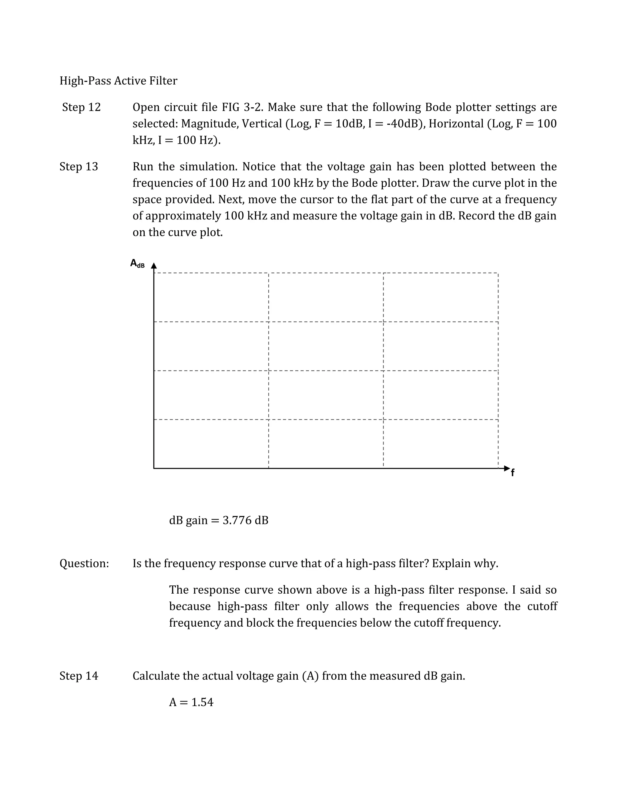
Download to read offline
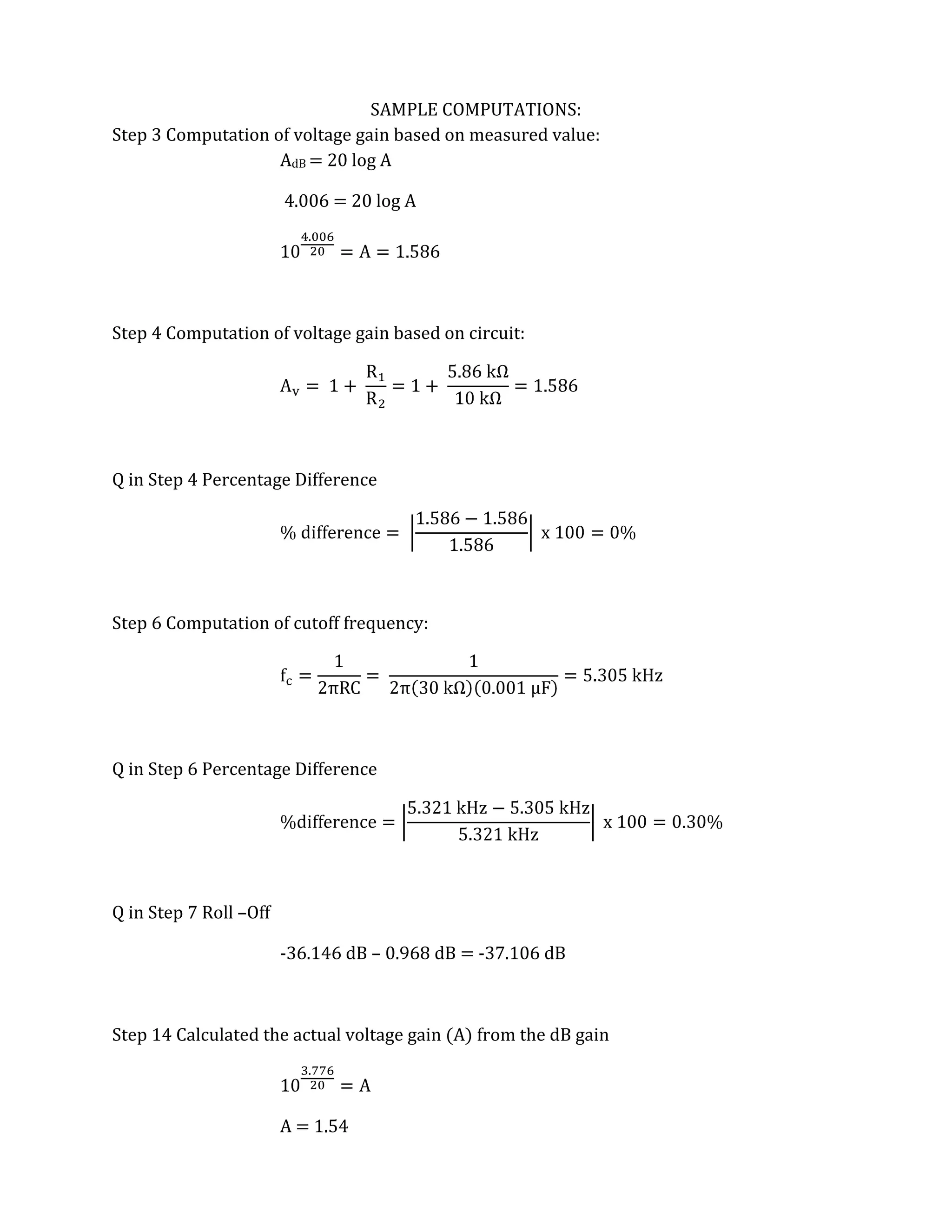


The dB gain at the 3dB point is: 1.006 dB The frequency at the 3dB point is: 100 Hz Step 6 Calculate the cutoff frequency (fc) based on the frequency at the 3dB point. fc = 100 Hz Question: How does the calculated cutoff frequency in Step 6 compare with the expected cutoff frequency based on the circuit component values? The calculated cutoff frequency in Step 6 is equal to the expected cutoff frequency based on the circuit component values, which is 100 Hz. Step 7 Determine the roll-off in dB/decade based on the Bode plot. Roll-off = -40 dB/decade


![Coded Agents – with UiPath SDK + LangGraph [Virtual Hands-on Workshop]](https://cdn.slidesharecdn.com/ss_thumbnails/codedagentsdeck-251215155422-5497c599-thumbnail.jpg?width=640&height=640&fit=bounds)


