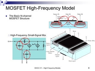
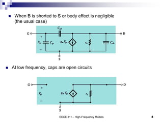
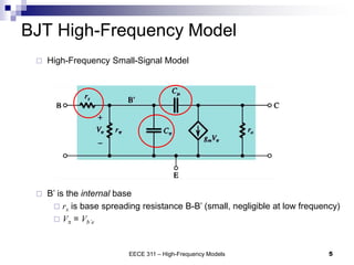
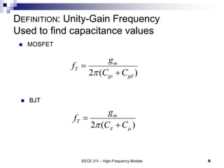
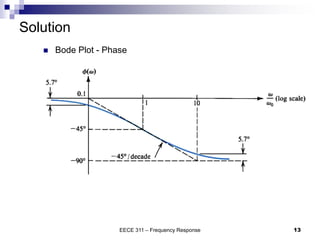
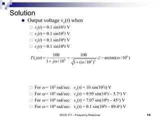
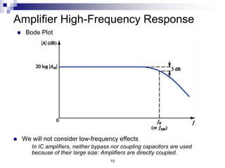
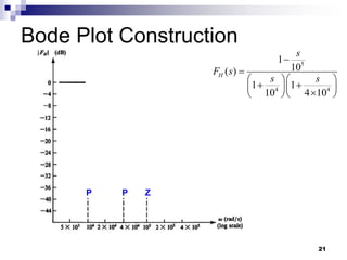
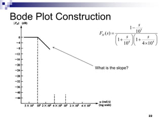
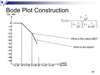
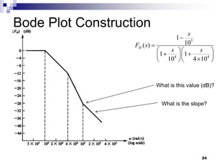
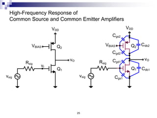
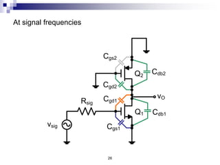
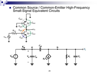
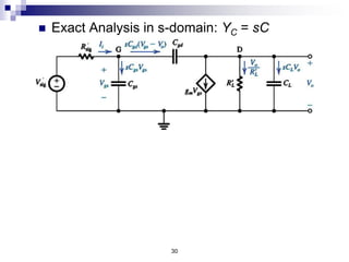
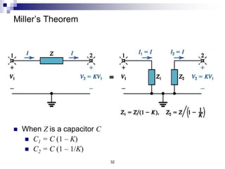
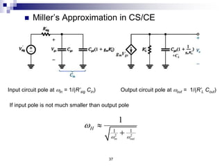
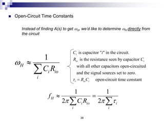
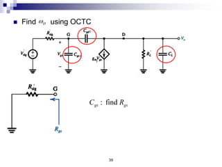
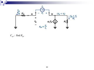
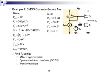
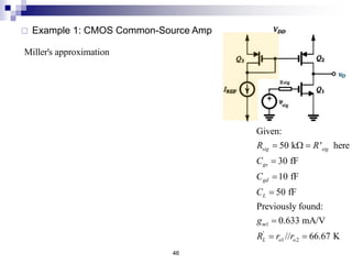
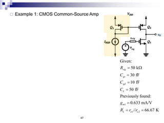
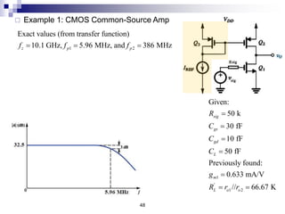
This document discusses the high-frequency response of electronic circuits such as amplifiers. It begins by introducing high-frequency small-signal models for MOSFETs and BJTs. It then defines the unity-gain frequency and describes how to find capacitance values using this frequency. The document provides an example of analyzing the effect of one capacitor on amplifier gain. It also discusses the frequency response of common source and common emitter amplifiers, showing their high-frequency small-signal equivalent circuits. Key aspects of amplifier frequency response like gain, poles, zeros, and Bode plots are covered.

1. EECE 311: Electronic Circuits
Part 2

2. AMPLIFIER FREQUENCY
RESPONSE
2

3.  High-Frequency Small-Signal Model
EECE 311 – High-Frequency Models 3
MOSFET High-Frequency Model
 The Basic N-channel
MOSFET Structure

4.  When B is shorted to S or body effect is negligible
(the usual case)
EECE 311 – High-Frequency Models 4
 At low frequency, caps are open circuits

5.  High-Frequency Small-Signal Model
EECE 311 – High-Frequency Models 5
BJT High-Frequency Model
 B’ is the internal base
 rx is base spreading resistance B-B’ (small, negligible at low frequency)
 Vp = Vb’e

6. EECE 311 – High-Frequency Models 6
DEFINITION: Unity-Gain Frequency
Used to find capacitance values
2 ( )
m
T
gs gd
g
f
C C
p


 MOSFET
 BJT
2 ( )
m
T
g
f
C C
p 
p



7. Frequency Response
 At low frequency
 capacitors are open-circuits (and inductors are short circuits)
 amplifier characteristics are not affected by frequency (no frequency-dependent elements)
 Capacitor impedance
 Changes with frequency: , Z(jw) = -j /wC (infinite at DC)
 As w increases, we need to study the “Frequency Response”
 Input is
 Output is since the system is linear
 How do A (magnitude) and f (phase) vary with frequency w?
EECE 311 – Frequency Response 7
1
( )
C
Z s
sC

sin( )
t
w
sin( )
A t
w f


8. Example – How does one capacitor affect
amplifier gain?
EECE 311 – Frequency Response 8
 Given: Blue block is the
amplifier
 Rs = 20 KW
 Ri = 100 KW
 Ci = 60 pF
  = 144 V/V
 Ro = 200 W
 RL = 1 KW
 Find:
 Vo/Vs
 Plot
 magnitude response
 phase response
 vo(t) when vs(t) = 0.1 sin10nt V
for n = 2, 5, 6, 8

9. Solution
EECE 311 – Frequency Response 9
i
i s
i s
Z
V V
Z R


 Express Vi as a function of Vs
1
1 1
1 1 ( )
i
i
i s s s
i s s i s i
R
Z
V V V V
Z R R Y R sC
  
   
1 1
1 1 ( // )
s
i
i i
R
R
s s i i s i s i
V R
V sR C R R sC R R
  
   
 Express Vo as a function of Vi
o
L L
o i
L o i L o
V
R R
V V
R R V R R
 
  
 

10. Solution
EECE 311 – Frequency Response 10
1
1 ( // )
o i
L
s L o i s i s i
V R
R
V R R R R sC R R

  
  
0
( )
1 /
o
s
V K
T s
V s w
 

 This is of the form:
K
1/w0
 Low-pass single-time-constant (LP-STC)
 K is the low-frequency gain
 w0 is the 3-dB frequency
1000 100K
144 100
1000 200 100K 20K
i
L
L o i s
R
R
K
R R R R

     
   
6
0 12 3
1 1
10 rad/sec
( // ) 60 10 (100//20) 10
i i s
C R R
w 
  
  

11. Review: Low-Pass Single Time Constant
 Gain (or Transfer) function:
 Low-frequency gain = K
 Upper 3-dB frequency = w0
 -20 dB/decade drop at high frequency (w >> w0)
 What is T at w0?
11
0
( )
1 /
o
s
V K
T s
V s w
 


12. Solution (continued)
EECE 311 – Frequency Response 12
 Bode Plot - Magnitude

13. Solution
EECE 311 – Frequency Response 13
 Bode Plot - Phase

14. Solution
EECE 311 – Frequency Response 14
 Output voltage vo(t) when
 vs(t) = 0.1 sin102t V
 vs(t) = 0.1 sin105t V
 vs(t) = 0.1 sin106t V
 vs(t) = 0.1 sin108t V
 For w = 102 rad/sec: vo(t) = 10 sin(102t) V
 For w = 105 rad/sec: vo(t) = 9.95 sin(105t – 5.7o) V
 For w = 106 rad/sec: vo(t) = 7.07 sin(106t – 45o) V
 For w = 108 rad/sec: vo(t) = 0.1 sin(108t – 89.4o) V
6
6 6 2
6
6 2
100 100
( ) arctan( /10 )
1 /10 1 ( /10 )
100
( ) 0.1 sin( arctan( /10 ))
1 ( /10 )
o
T j
j
v t t
w w
w w
w w
w
   
 
  


15. 15
Amplifier High-Frequency Response
 We will not consider low-frequency effects
In IC amplifiers, neither bypass nor coupling capacitors are used
because of their large size: Amplifiers are directly coupled.
 Bode Plot

16. 16
0
1 2
1 2
1 2
1 2
( ) ( )
( ) 1
lim
1 1 ... 1
( )
1 1 ... 1
, ... are the zero frequencies and can be positive, negative or infinite.
, .
M H
H
s
Z Z Zn
H
P P Pn
Z Z Zn
P P
A s A F s
F s
s s s
F s
s s s
w w w
w w w
w w w
w w

 

 
  
  
 
  
    

 
  
  
 
  
    
.. are the pole frequencies and are positive and real.
Pn
w
 The High-Frequency Gain Function

17. 17
if wP 1
<<wP 2
,… ,wPn
, wZ 1
, wZ 2
,… , wZn
then FH
(s) @
1
1+
s
wP 1
(Low Pass STC)
wH
=wP 1
Þ f H
=
wP 1
2p
 The Dominant Pole Approximation
H 2 2 2 2
1 2 1 2
1 1 1 1
1 ... 2 ...
P P Z Z
w
w w w w
   
     
   
   
 Better Approximation
If one pole is obviously smaller than the other zeroes and poles.
wp1 is 2 octaves down
(less by a factor of 4)

18. 18
2 2
1 2
2 2
1 2
2
2 2 2 2 2
1 2 1
1
( )
2
1 . 1 ...
1
2
1 . 1 ...
let
1 1 ... 1 2 1 ... 1
H H
H H
Z Z
H H
P P
H
P P Pn Z Zn
F j
x
x x x x x
w
w w
w w
w w
w w
w
w w w w w

   
 
   
   

   
 
   
   

   
    
     
   
    
    
   
 The Exact Solution: Solve |A|=|AM|/√2
ωH = √x

19. 19
 Example: Find H
w
5
4 4
1
10
( )
1 1
10 4 10
H
s
F s
s s


  
 
  

  
5
1
2
4
1
4
2
10 rad/sec
10 rad/sec
4 10 rad/sec
Z
Z
P
P
w
w
w
w
 
 

 
 Given:
 Solution:
 Dominant Pole?
4
10 rad/sec
H
w 
 Better Approximation:
H 2 2 2 2
1 2 1 2
1 1 1 1
1 2 9800 rad/sec
P P Z Z
w
w w w w
   
    
   
   
 Exact Solution:
2 2 2
1 2 1
1 1 2 1
9573 rad/sec
P P Z
H
x x x
x
w w w
w
    
   
    
    
 

20. 20
 Example: Magnitude Bode Plot
5
4 4
1
10
( )
1 1
10 4 10
H
s
F s
s s


  
 
  

  
 Given:
Pole:
slope 20 dB/decade
Zero:
slope 20 dB/decade
 
 

21. Bode Plot Construction
21
5
4 4
1
10
( )
1 1
10 4 10
H
s
F s
s s


  
 
  

  
P P Z

22. Bode Plot Construction
22
5
4 4
1
10
( )
1 1
10 4 10
H
s
F s
s s


  
 
  

  
What is the slope?

23. Bode Plot Construction
23
5
4 4
1
10
( )
1 1
10 4 10
H
s
F s
s s


  
 
  

  
What is the slope?
What is this value (dB)?

24. Bode Plot Construction
24
5
4 4
1
10
( )
1 1
10 4 10
H
s
F s
s s


  
 
  

  
What is the slope?
What is this value (dB)?

25. 25
High-Frequency Response of
Common Source and Common Emitter Amplifiers
vsig
Rsig
VDD
vI
Q1
vO
Q2
VBIAS
Rsig
vsig
VDD
Q1
vO
Q2
VBIAS Cdb2
Cdb1
Cgd2
Cgs2
Cgs1
Cgd1

26. 26
At signal frequencies
Rsig
vsig
Q1
vO
Q2
Cdb2
Cdb1
Cgd2
Cgs2
Cgs1
Cgd1

27. 27
High-Frequency Response of
Common Source and Common Emitter Amplifiers
 High-Frequency Small-Signal Equivalent Circuits
CS:
CE:

28.  RL represents the output resistance of the active load and any load resistance
 CL represents the total capacitance between drain (or collector) and ground. It also
includes the input capacitance of a succeeding amplifier stage, and parasitic/load
capacitances.
 We will analyze the CS circuit only since the analysis of the CE amplifier is exactly
the same after relabeling
28
to , to , to
gs gd gs
C C C C V V
p  p
 
'
'
//
sig sig
sig x
sig x sig
r
V V
r R r
R r R r
p
p
p
 
 
 
and replacing and by:
sig sig
V R
Thevenin equivalent
for circuit composed
of Vsig, Rsig, rx, and rp

29. 29
 Common Source / Common-Emitter High-Frequency
Small-Signal Equivalent Circuits
Rsig
vsig
Q1
vO
Q2
Cdb2
Cdb1
Cgd2
Cgs2
Cgs1
Cgd1

30. 30
 Exact Analysis in s-domain: YC = sC
 
 
'
' '
KCL at drain:
KVL at input:
0
KCL at gate:
o
gd gs o m gs L o
L
sig sig i gs
i gs gs gd gs o
V
sC V V g V sC V
R
V R I V
I sC V sC V V
   
  
  

31.  
   
   
'
' ' ' ' 2 ' '
' 2
1 2
1 2
1
1
1 1
1 1
1
1 1
1
gd
m L
m
o
sig gs gd m L sig L gd L L gd gs L gd sig L
M M
Z Z
o m
Z
sig gd
P P
P
C
g R s
g
V
V s C C g R R C C R s C C C C C R R
s s
A A
V g
V b s b s C
s s
s
w w
w
w w
w
 
 
 
 

   
       
 
 
   
 
   
   
   
    
 
  
  
 



   
   
 
2
2 1 2 1 2
1 ' ' '
' ' '
2 ' '
1 1 1
1 1
1
1
1
P P P P P
P
gs gd m L sig L gd L
gs gd m L sig L gd L
P
L gd gs L gd sig L
s
s s
C C g R R C C R
C C g R R C C R
C C C C C R R
w w w w w
w
w
   
    
   
   
 
 
   
 
 
   
 
 
 
 
 
1 2
negligible ( 0) if P P
w w
 
31
•Low frequency
gain is –gmR’L
•Zero frequency
gm/Cgd is very high
•What is the 3-dB
frequency?

32. 32
Miller’s Theorem
 When Z is a capacitor C
 C1 = C (1 – K)
 C2 = C (1 – 1/K)

33. 33
 Example 2: Find / and .
o sig H
V V w
 Given:
 Solution using Miller
1 pF
Z 
100
K   100
o i
V V
 
  
1
1
1
9
1
1
1 1
1
1 10 k 101 p
100
100
1 (1010 n) 1
10
157.6 kHz
1010 2
i
sig sig
sig
i
sig
o m
o i
sig
H
H
H H
V sC
V sC R
R
sC
V
V s
V A
V V
s
V s
f
w
w
w
p
 





    
 
    
1
2
101pF
1.01pF
C
C



34. 34
 Find using Miller’s Theorem
H
w

35. 35
 Miller’s Approximation in CS/CE
 
'
1
in gs gd m L
C C C g R
  
'
At midband, o
m L
gs
V
K g R
V
  
The input circuit and the output circuit are low-pass
RC circuits
What is the pole frequency for a simple RC circuit?
Cout
=Cgd
1+
1
gm
RL
'
æ
è
ç
ç
ö
ø
÷
÷+CL
+CL

36. 36
 Miller’s Approximation in CS/CE
 
' ' '
1 1
1
H
sig in sig gs gd m L
R C R C C g R
w  
 
 
 
'
1
o m
m m L
sig
H
V A
A g R
s
V
w
  

Input circuit pole at 1/(R’sig Cin) Output circuit pole at 1/(R’L Cout)
Usually input circuit determines high frequency response
+CL

37. 37
 Miller’s Approximation in CS/CE
Input circuit pole at win = 1/(R’sig Cin) Output circuit pole at wout = 1/(R’L Cout)
2 2
1 1
1
in out
H
w w
w 

If input pole is not much smaller than output pole
+CL

38. 38
 Open-Circuit Time Constants
Instead of finding A(s) to get wH, we’d like to determine wH directly from
the circuit
1
H
i io
i
C R
w 

is capacitor " " in the circuit.
is the resistance seen by capacitor
with all other capacitors open-circuited
and the signal sources set to zero.
open-circuit time constant
i
io i
i io i
C i
R C
R C
 
1 1
2 2
H
i io i
i i
f
C R
p p 
 
 

39. 39
 Find using OCTC
H
w
'
'
: find
gs gs sig
gs gs gs gs sig
C R R
C R C R


  

40. 40
 
'
1 1
' '
1
' '
1
: find
' '
' '
' '
gd gd
gs x sig
gs x
o
x m gs m gs
L L
x
gd sig L m sig L
x
gd gd gd gd sig L m sig L
C R
V I R
V V
V
I g V g V
R R
V
R R R g R R
I
C R C R R g R R

 

   
   
    

41.  Frequently-used resistance calculation
41
RX RY
gmVX
VX
+
-
RXY
(1 ) where
(1 ) where
XY X Y m X Y
XY Y X Y Y m Y
XY X Y X X m X
R R R g R R
R R R g R
R R R g R
 
 
  
   
   

42. 42
 Find using OCTC (cont’d)
H
w
: find
L CL
C R

43. 9
1 10
rad/sec
80 1000 1080
H
w  

43
Open-Circuit Time Constants (cont’d)
'
' ' ' '
'
gs gs sig
gd gd sig L m sig L
L CL L
C R R
C R R R g R R
C R R
 
   
 
gs gs gs
gd gd gd
cl L CL
C R
C R
C R






1
H
gs gd cl
w
  

 
 Numberical Example: Find .
H
w
1 pF
1pF
gs
gd
C
C


80 k neglect
1000 k
gs L
gd
R C
R
 W
 W
 Given:
 Solution:
80 ns
1000 ns
gs gs gs
gd gd gd
C R
C R


 
 
OCTC allows us to
determine the circuit
component(s) that
limit the value of wH

44.  
' ' '
' ' '
L
gs gd C
gs sig gd sig L m sig L L L
C R C R R g R R C R
   
  
    
44
 Open-Circuit Time Constants (cont’d)
 
' ' '
1
' ' '
H
gs sig gd sig L m sig L L L
C R C R R g R R C R
w 
   
'
1
o m
m m L
sig
H
V A
A g R
s
V
w
  


45. 45
 Example 1: CMOS Common-Source Amp
' 2
' 2
Given
3V
200 A/V
65 A/V
10 for all MOSFETs
0.6V
20V
10V
100 A
DD
n
p
W
L
tn tp
An
Ap
REF
V
k
k
V V
V
V
I







 



 Find fH using:
 Miller’s approximation
 Open-circuit time constants (OCTC)
 Transfer function
Given
50 k
30 fF
10 fF
50 fF
sig
gs
gd
L
R
C
C
C
 W




46. '
1
'
1
Miller's approximation
input pole frequency:
(1 ) 30 43.2 10 462 fF
1
6.89 MHz
2 '
output pole frequency:
1 1
1 10 1 50 60.24 fF
42.2
1
39
2 '
in gs m L gd
in
in sig
out gd L
m L
out
out L
C C g R C
f
C R
C C C
g R
f
C R
p
p
      
 
   
      
   
 
 
  .6 MHz
input pole is dominant:
6.89 MHz
H
f 
46
 Example 1: CMOS Common-Source Amp
1
'
1 2
Given:
50 k ' here
30 fF
10 fF
50 fF
Previously found:
0.633 mA/V
// 66.67 K
sig sig
gs
gd
L
m
L o o
R R
C
C
C
g
R r r
 W 




 

47. 47
 Example 1: CMOS Common-Source Amp
1
'
1 2
Given:
50 k
30 fF
10 fF
50 fF
Previously found:
0.633 mA/V
// 66.67 K
sig
gs
gd
L
m
L o o
R
C
C
C
g
R r r
 W




 
' '
1
'
OCTC
' 50k
' (1 ) 50 43.2 66.67 2226.67k
66.67k
30 50 10 2226.67 50 66.67
1500 22266.7 3333.3
1
5.87 MHz
2
L
L
gs sig
gd sig m L L
C L
H gs gs gd gd L C
H
H
R R
R R g R R
R R
C R C R C R
f

p
 
      
 
  
     
  
 

48. 48
 Example 1: CMOS Common-Source Amp
1
'
1 2
Given:
50 k
30 fF
10 fF
50 fF
Previously found:
0.633 mA/V
// 66.67 K
sig
gs
gd
L
m
L o o
R
C
C
C
g
R r r





 
1 2
1
1
Exact values (from transfer function)
10.1 GHz, 5.96 MHz, and 386 MHz
is a dominant pole
5.96 MHz
Error in Miller's approximation = +15.6%
Error in OCTC approximation = 1.51%
z p p
p
H p
f f f
f very
f f
  
 


49.  Example 2: CMOS Common-Source Cascade
 What is the overall low-frequency gain if the per-stage gain is –42?
 What is the 3-dB frequency if the per-stage 3-dB fH is 6 MHz?

50. Solution
50

51. Example 3: Common-Emitter Amplifier
 Find the 3-dB frequency
fH using Miller’s approximation
 Assume that the input circuit
determines the value of fH
51
vi
Q3
IREF
Q2
Q1
vo
VCC
Rsig
vsig

52. Solution
52