mobile radio environment

1. MOBILE RADIO ENVIRONMENT
AND SIGNAL DISTURBANCE
1
Dr.C.Helen Sulochana
Professor/ECE
St.Xviers Catholic College of Engg, Chunkankadai

2. 2

6. Radio wave propogation
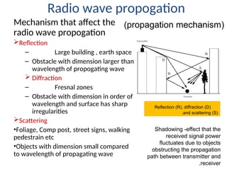
Mechanism that affect the
radio wave propogation
Reflection
– Large building , earth space
– Obstacle with dimension larger than
wavelength of propogating wave
 Diffraction
– Fresnal zones
– Obstacle with dimension in order of
wavelength and surface has sharp
irregularities
Scattering
•Foliage, Comp post, street signs, walking
pedestrain etc
•Objects with dimension small compared
to wavelength of propagating wave
Reflection (R), diffraction (D)
and scattering (S)
.
(
propagation mechanism
)
Shadowing -effect that the
received signal power
fluctuates due to objects
obstructing the propagation
path between transmitter and
receiver
.

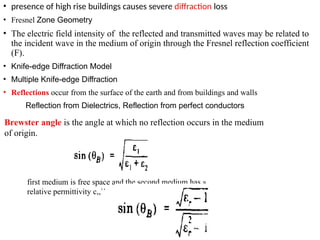
7. • presence of high rise buildings causes severe diffraction loss
• Fresnel Zone Geometry
• The electric field intensity of the reflected and transmitted waves may be related to
the incident wave in the medium of origin through the Fresnel reflection coefficient
(F).
• Knife-edge Diffraction Model
• Multiple Knife-edge Diffraction
• Reflections occur from the surface of the earth and from buildings and walls
Reflection from Dielectrics, Reflection from perfect conductors
Brewster angle is the angle at which no reflection occurs in the medium
of origin.
first medium is free space and the second medium has a
relative permittivity c,,``

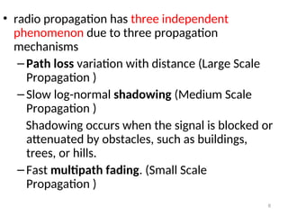
8. • radio propagation has three independent
phenomenon due to three propagation
mechanisms
–Path loss variation with distance (Large Scale
Propagation )
–Slow log-normal shadowing (Medium Scale
Propagation )
Shadowing occurs when the signal is blocked or
attenuated by obstacles, such as buildings,
trees, or hills.
–Fast multipath fading. (Small Scale
Propagation )
8

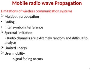
9. Mobile radio wave Propagation
Limitations of wireless communication systems
 Multipath propagation
• Fading
• Inter symbol interference
 Spectral limitation
- Radio channels are extremely random and difficult to
analyse
 Limited Energy
 User mobility
-signal fading occurs
9

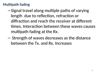
10. Multipath fading
–Signal travel along multiple paths of varying
length due to reflection, refraction or
diffraction and reach the receiver at different
times. Interaction between these waves causes
multipath fading at the Rx.
– Strength of waves decreases as the distance
between the Tx. and Rx. Increases
10

11. WIRELESS CHANNELS
WIRELESS CHANNELS
11

12. • Large Scale Path Loss: Introduction To Radio Wave
Propagation - Free Space Propagation Model – Three
Basic Propagation Mechanism: Reflection – Brewster
Angle- Diffraction, Scattering. Small Scale Fading And
Multipath: Small Scale Multipath Propagation, Factors
Influencing Small-Scale Fading, Doppler Shift,
Coherence Bandwidth, Doppler Spread And Coherence
Time. Types Of Small- Scale Fading: Fading Effects
Due To Multipath Time Delay Spread, Fading Effects
Due To Doppler Spread.
12
CO-Develop path loss models for wireless channels
.

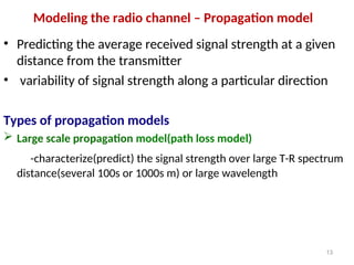
13. Modeling the radio channel – Propagation model
• Predicting the average received signal strength at a given
distance from the transmitter
• variability of signal strength along a particular direction
Types of propagation models
 Large scale propagation model(path loss model)
-characterize(predict) the signal strength over large T-R spectrum
distance(several 100s or 1000s m) or large wavelength
13

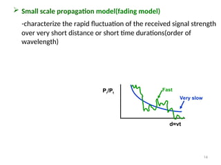
14.  Small scale propagation model(fading model)
-characterize the rapid fluctuation of the received signal strength
over very short distance or short time durations(order of
wavelength)
14
Pr/Pt
d=vt
Very slow
Fast

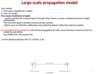
15. Large scale propagation model
Two models
1. Free space model(Line of sight)
2. Two ray model
Free space model(Line of sight)
-used to predict the received signal strength when there is a clear, unobstructed line of sight
propagation
-The received signal is directly received at the receiver
- effects such as reflection, diffraction and scattering doesn’t affect the signal reception.
Line-of-sight(LoS) propagation is the direct propagation of radio waves between antennas that are
visible to each other.
-eg satellite link, microwave link
Let the distance between the Tx. and Rx. is d
15

16. 16
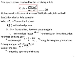
Free space power received by the receiving ant. Is
…………(1)
Pr decays with distance at a rate of 20dB/decade, falls with d2
Eqn(1) is called as Friis equation
Where Pt -- Transmitted power,
Pr(d) -- Received power
Gt , Gr - Transmitter, Receiver antenna gain
L -system loss factor -transmission line attenuation,
fiber loss and ant. Loss
-wavelength , , -angular frequency in radians
f –frequency, c- velocity of light
Gain of the ant.
- effective aperture of the ant.

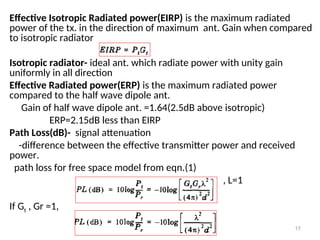
17. Effective Isotropic Radiated power(EIRP) is the maximum radiated
power of the tx. in the direction of maximum ant. Gain when compared
to isotropic radiator
Isotropic radiator- ideal ant. which radiate power with unity gain
uniformly in all direction
Effective Radiated power(ERP) is the maximum radiated power
compared to the half wave dipole ant.
Gain of half wave dipole ant. =1.64(2.5dB above isotropic)
ERP=2.15dB less than EIRP
Path Loss(dB)- signal attenuation
-difference between the effective transmitter power and received
power.
path loss for free space model from eqn.(1)
, L=1
If Gt , Gr =1,
17

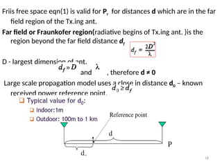
18. Friis free space eqn(1) is valid for Pr for distances d which are in the far
field region of the Tx.ing ant.
Far field or Fraunkofer region(radiative begins of Tx.ing ant. )is the
region beyond the far field distance df
D - largest dimension of ant.
and , therefore d ≠ 0
Large scale propagation model uses a close in distance d0 – known
received power reference point,
18

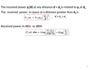
19. The received power pr(d) at any distance d > d0 is related to pr at d0
The received power in space at a distance greater than d0 is
,
Received power in dBm or dBW
19

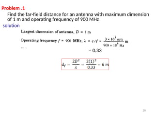
20. Problem .1
Find the far-field distance for an antenna with maximum dimension
of 1 m and operating frequency of 900 MHz
solution
= 0.33
20

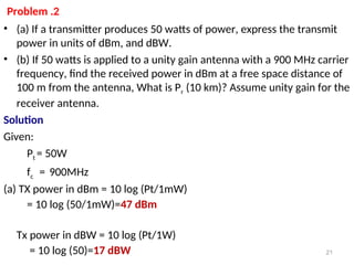
21. Problem .2
• (a) If a transmitter produces 50 watts of power, express the transmit
power in units of dBm, and dBW.
• (b) If 50 watts is applied to a unity gain antenna with a 900 MHz carrier
frequency, find the received power in dBm at a free space distance of
100 m from the antenna, What is Pr (10 km)? Assume unity gain for the
receiver antenna.
Solution
Given:
Pt = 50W
fc = 900MHz
(a) TX power in dBm = 10 log (Pt/1mW)
= 10 log (50/1mW)=47 dBm
Tx power in dBW = 10 log (Pt/1W)
= 10 log (50)=17 dBW 21

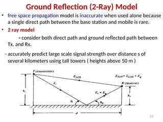
22. Ground Reflection (2-Ray) Model
• free space propagation model is inaccurate when used alone because
a single direct path between the base station and mobile is rare.
• 2 ray model
- consider both direct path and ground reflected path between
Tx. and Rx.
- accurately predict large scale signal strength over distance s of
several kilometers using tall towers ( heights above 50 m )
23

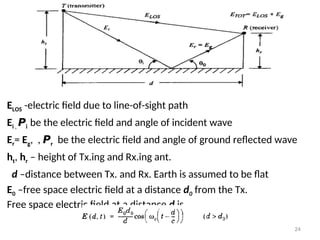
23. ELOS -electric field due to line-of-sight path
Ei , 𝞠i be the electric field and angle of incident wave
Er= Eg, , 𝞠r be the electric field and angle of ground reflected wave
ht, hr – height of Tx.ing and Rx.ing ant.
d –distance between Tx. and Rx. Earth is assumed to be flat
E0 –free space electric field at a distance d0 from the Tx.
Free space electric field at a distance d is
24

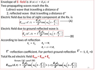
24. Envelope of E- field is
Two propagating waves reach the Rx.
1.direct wave that travelling a distance d’
2. reflected wave that travelling a distance d’’
Electric field due to line of sight component at the Rx. is
---------(A)
Electric field due to ground reflected wave is
------(B)
According to laws of reflection
-reflection coefficient. For perfect ground reflection = -1, Et =0
Total Rx.ed electric field ETOT = ELOS + Eg
from (A) and (B)
25

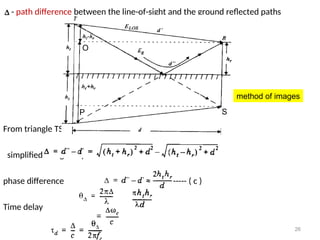
25. - path difference between the line-of-sight and the ground reflected paths
From triangle TSP and TRO
simplified using a Taylor series
phase difference = 4 --------------- ( c )
Time delay
26
method of images
O
S
P

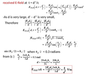
26. received E-field at t = d‘’/c
-
-As d is very large, d' – d’’ is very small,
Therefore
when < 0.3 radians
from (c )

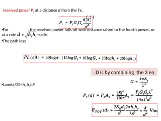
27. received power Pr at a distance d from the Tx.
……… ( D )
•For , the received power falls off with distance raised to the fourth power, or
at a rate of 40 dB/ decade.
•The path loss
•Lamda/20=ht hr/d2
28
D is by combining the 3 en
.

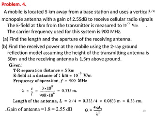
28. Problem. 4.
A mobile is located 5 km away from a base station and uses a vertical
monopole antenna with a gain of 2.55dB to receive cellular radio signals
The E-field at 1km from the transmitter is measured to be .
The carrier frequency used for this system is 900 MHz.
(a) Find the length and the aperture of the receiving antenna.
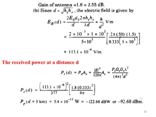
(b) Find the received power at the mobile using the 2-ray ground
reflection model assuming the height of the transmitting antenna is
50m and the receiving antenna is 1.5m above ground.
29
Gain of antenna =1.8 = 2.55 dB
.

29. 30
The received power at a distance d

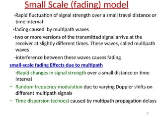
30. Small Scale (fading) model
-Rapid fluctuation of signal strength over a small travel distance or
time interval
-fading caused by multipath waves
-two or more versions of the transmitted signal arrive at the
receiver at slightly different times. These waves, called multipath
waves
-interference between these waves causes fading
small-scale fading Effects due to multipath
-Rapid changes in signal strength over a small distance or time
interval
– Random frequency modulation due to varying Doppler shifts on
different multipath signals
– Time dispersion (echoes) caused by multipath propagation delays
31

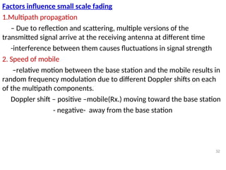
31. Factors influence small scale fading
1.Multipath propagation
– Due to reflection and scattering, multiple versions of the
transmitted signal arrive at the receiving antenna at different time
-interference between them causes fluctuations in signal strength
2. Speed of mobile
–relative motion between the base station and the mobile results in
random frequency modulation due to different Doppler shifts on each
of the multipath components.
Doppler shift – positive –mobile(Rx.) moving toward the base station
- negative- away from the base station
32

32. 3. Speed of surrounding
– if the surrounding objects move at a greater rate than the mobile,
Doppler shift introduced on multipath components is considered.
4. The transmission bandwidth of the signal
•—If signal BW is greater than the multipath channel BW, the received
signal will be distorted,
- but the received signal strength will not fade much over a local
area
33

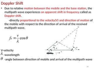
33. Doppler Shift
• Due to relative motion between the mobile and the base station, the
multipath wave experiences an apparent shift in frequency called as
Doppler shift.
-directly proportional to the velocity(V) and direction of motion of
the mobile with respect to the direction of arrival of the received
multipath wave.
V-velocity
-wavelength
-angle between direction of mobile and arrival of the multipath wave
34


cos
v
fd 



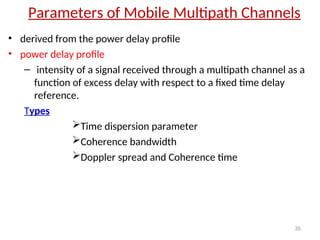
34. Parameters of Mobile Multipath Channels
• derived from the power delay profile
• power delay profile
– intensity of a signal received through a multipath channel as a
function of excess delay with respect to a fixed time delay
reference.
Types
Time dispersion parameter
Coherence bandwidth
Doppler spread and Coherence time
35

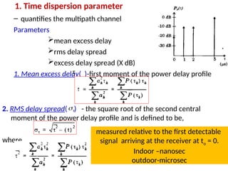
35. 1. Time dispersion parameter
– quantifies the multipath channel
Parameters
mean excess delay
rms delay spread
excess delay spread (X dB)
1. Mean excess delay( )-first moment of the power delay profile
2. RMS delay spread( ) - the square root of the second central
moment of the power delay profile and is defined to be,
where
36
τ


measured relative to the first detectable
signal arriving at the receiver at to = 0.
Indoor –nanosec
outdoor-microsec

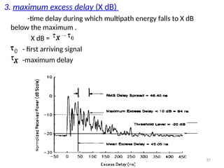
36. 3. maximum excess delay (X dB)
-time delay during which multipath energy falls to X dB
below the maximum .
X dB =
- first arriving signal
-maximum delay
37

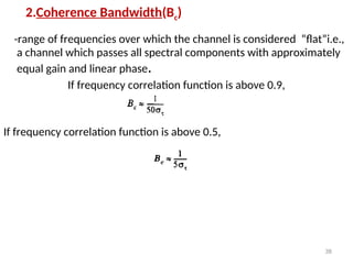
37. 2.Coherence Bandwidth(Bc)
-range of frequencies over which the channel is considered “flat”i.e.,
a channel which passes all spectral components with approximately
equal gain and linear phase.
If frequency correlation function is above 0.9,
If frequency correlation function is above 0.5,
38

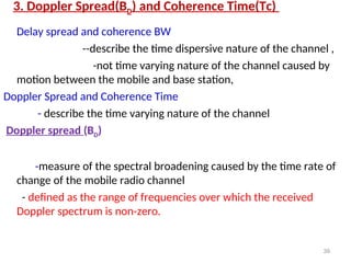
38. 3. Doppler Spread(BD) and Coherence Time(Tc)
Delay spread and coherence BW
--describe the time dispersive nature of the channel ,
-not time varying nature of the channel caused by
motion between the mobile and base station,
Doppler Spread and Coherence Time
- describe the time varying nature of the channel
Doppler spread (BD)
-measure of the spectral broadening caused by the time rate of
change of the mobile radio channel
- defined as the range of frequencies over which the received
Doppler spectrum is non-zero.
39

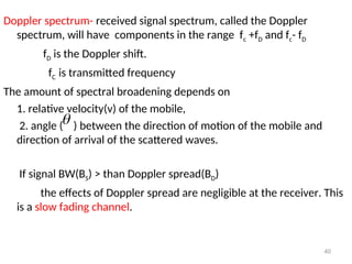
39. Doppler spectrum- received signal spectrum, called the Doppler
spectrum, will have components in the range fc +fD and fc- fD
fD is the Doppler shift.
fC is transmitted frequency
The amount of spectral broadening depends on
1. relative velocity(v) of the mobile,
2. angle ( ) between the direction of motion of the mobile and
direction of arrival of the scattered waves.
If signal BW(BS) > than Doppler spread(BD)
the effects of Doppler spread are negligible at the receiver. This
is a slow fading channel.
40


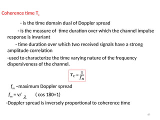
40. Coherence time Tc
- is the time domain dual of Doppler spread
- is the measure of time duration over which the channel impulse
response is invariant
- time duration over which two received signals have a strong
amplitude correlation
-used to characterize the time varying nature of the frequency
dispersiveness of the channel.
fm –maximum Doppler spread
fm = v/ ( cos 180=1)
-Doppler spread is inversely proportional to coherence time
41


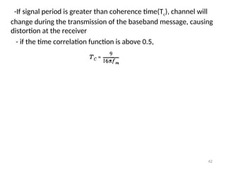
41. -If signal period is greater than coherence time(Tc), channel will
change during the transmission of the baseband message, causing
distortion at the receiver
- if the time correlation function is above 0.5,
42

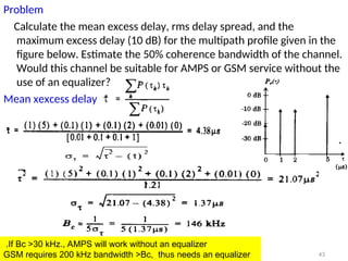
42. Problem
Calculate the mean excess delay, rms delay spread, and the
maximum excess delay (10 dB) for the multipath profile given in the
figure below. Estimate the 50% coherence bandwidth of the channel.
Would this channel be suitable for AMPS or GSM service without the
use of an equalizer?
Mean xexcess delay
43
If Bc >30 kHz., AMPS will work without an equalizer
.
GSM requires 200 kHz bandwidth >Bc, thus needs an equalizer

43. Problem
• Determine the proper spatial sampling interval required to make
small-scale propagation measurements which assume that
consecutive samples are highly correlated in time. How many
samples will be required over 10 m travel distance if fc = 1900 MHz
and v = 50 in/s. How long would it take to make these
measurements, assuming they could be made in real time from a
moving vehicle? What is the Doppler spread BD for the channel?
44

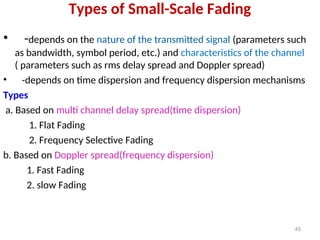
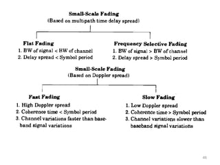
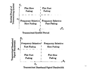
44. Types of Small-Scale Fading
• -depends on the nature of the transmitted signal (parameters such
as bandwidth, symbol period, etc.) and characteristics of the channel
( parameters such as rms delay spread and Doppler spread)
• -depends on time dispersion and frequency dispersion mechanisms
Types
a. Based on multi channel delay spread(time dispersion)
1. Flat Fading
2. Frequency Selective Fading
b. Based on Doppler spread(frequency dispersion)
1. Fast Fading
2. slow Fading
45

45. 46

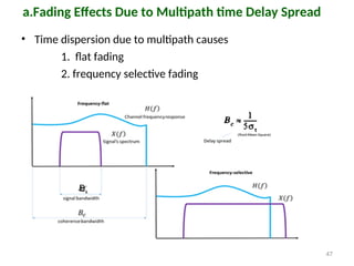
46. • Time dispersion due to multipath causes
1. flat fading
2. frequency selective fading
47
a.Fading Effects Due to Multipath time Delay Spread
Bs

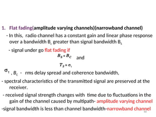
47. 1. Flat fading(amplitude varying channels)(narrowband channel)
- In this, radio channel has a constant gain and linear phase response
over a bandwidth Bc greater than signal bandwidth BS
- signal under go flat fading if
and
, BC - rms delay spread and coherence bandwidth,
- spectral characteristics of the transmitted signal are preserved at the
receiver.
- received signal strength changes with time due to fluctuations in the
gain of the channel caused by multipath- amplitude varying channel
-signal bandwidth is less than channel bandwidth-narrowband channel
48

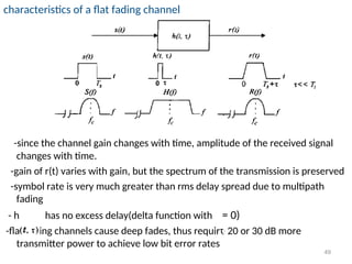
48. characteristics of a flat fading channel
-since the channel gain changes with time, amplitude of the received signal
changes with time.
-gain of r(t) varies with gain, but the spectrum of the transmission is preserved
-symbol rate is very much greater than rms delay spread due to multipath
fading
- h has no excess delay(delta function with = 0)
-flat fading channels cause deep fades, thus require 20 or 30 dB more
transmitter power to achieve low bit error rates
49

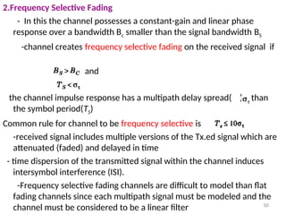
49. 2.Frequency Selective Fading
- In this the channel possesses a constant-gain and linear phase
response over a bandwidth Bc smaller than the signal bandwidth BS
-channel creates frequency selective fading on the received signal if
and
the channel impulse response has a multipath delay spread( ) > than
the symbol period(TS)
Common rule for channel to be frequency selective is
-received signal includes multiple versions of the Tx.ed signal which are
attenuated (faded) and delayed in time
- time dispersion of the transmitted signal within the channel induces
intersymbol interference (ISI).
-Frequency selective fading channels are difficult to model than flat
fading channels since each multipath signal must be modeled and the
channel must be considered to be a linear filter 50

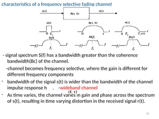
50. characteristics of a frequency selective fading channel
- signal spectrum S(f) has a bandwidth greater than the coherence
bandwidth(Bc) of the channel.
-channel becomes frequency selective, where the gain is different for
different frequency components
- bandwidth of the signal s(t) is wider than the bandwidth of the channel
impulse response h . -wideband channel
- As time varies, the channel varies in gain and phase across the spectrum
of s(t), resulting in time varying distortion in the received signal r(t).
51

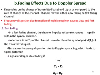
51. b.Fading Effects Due to Doppler Spread
• Depending on the change of transmitted baseband signal as compared to the
rate of change of the channel , channel may be either slow fading or fast fading
channel
• Frequency dispersion due to motion of mobile receiver causes slow and fast
fading
3. Fast fading
-In a fast fading channel, the channel impulse response changes rapidly
within the symbol duration.
-coherence time(TC) of the channel is smaller than the symbol period(TS) of
the transmitted signal.
-This causes frequency dispersion due to Doppler spreading, which leads to
signal distortion
-a signal undergoes fast fading if
and
52

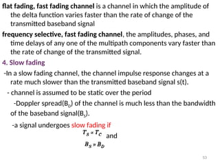
52. flat fading, fast fading channel is a channel in which the amplitude of
the delta function varies faster than the rate of change of the
transmitted baseband signal
frequency selective, fast fading channel, the amplitudes, phases, and
time delays of any one of the multipath components vary faster than
the rate of change of the transmitted signal.
4. Slow fading
-In a slow fading channel, the channel impulse response changes at a
rate much slower than the transmitted baseband signal s(t).
- channel is assumed to be static over the period
-Doppler spread(BD) of the channel is much less than the bandwidth
of the baseband signal(BS).
-a signal undergoes slow fading if
and
53

53. 54

54. Link Budget Design using Path Loss Models
- radio propagation models are derived using analytical(theory based)
and empirical(measurement based)methods.
- empirical approach is based on measurements carried out in the
complex environments containing more obstacles. These are called
path loss models. It gives the amount of loss encountered by the
signal along its path.
- analytical models are theory based and include some analytical
expression to calculate the path loss
Practical path loss models are
1. Log-distance Path Loss Model
2. Log-normal Shadowing
55

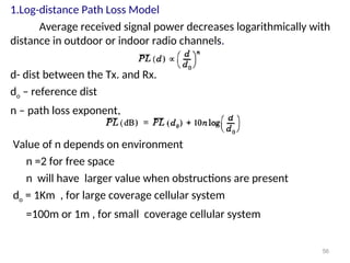
55. 1.Log-distance Path Loss Model
Average received signal power decreases logarithmically with
distance in outdoor or indoor radio channels.
d- dist between the Tx. and Rx.
do – reference dist
n – path loss exponent,
Value of n depends on environment
n =2 for free space
n will have larger value when obstructions are present
do = 1Km , for large coverage cellular system
=100m or 1m , for small coverage cellular system
56

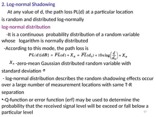
56. 2. Log-normal Shadowing
At any value of d, the path loss PL(d) at a particular location
is random and distributed log-normally
log-normal distribution
-It is a continuous probability distribution of a random variable
whose logarithm is normally distributed
-According to this mode, the path loss is
-zero-mean Gaussian distributed random variable with
standard deviation
- log-normal distribution describes the random shadowing effects occur
over a large number of measurement locations with same T-R
separation
•-Q-function or error function (erf) may be used to determine the
probability that the received signal level will be exceed or fall below a
particular level 57

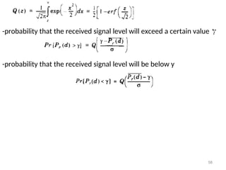
57. -probability that the received signal level will exceed a certain value
-probability that the received signal level will be below y
58

58. Outdoor Propagation Models
1. Longley-RIce Model
-applicable to point-to-point communication systems in the frequency
range from 40 MHz to 100 GHz, over different kinds of terrain
- Longley-Rice method operates in two modes.
a. When a detailed terrain path profile is available, the path-specific
parameters(horizon distance of the antennas, horizon elevation angle,
angular trans-horizon distance, terrain irregularity)can be easily
determined and the prediction is called a point-to-point mode prediction.
b. if the terrain path profile is not available, the Longley-Rice method
provides techniques to estimate the path-specific parameters, and such a
prediction is called an area mode prediction.
• does not provide a way of determining corrections due to environmental
factors
2. Durkin's Model
59

59. 3. Okumura Model
-most widely used models in urban areas for frequencies 150MHz to
1920 MHz and distances of 1 km to 100 km
60