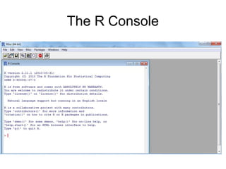
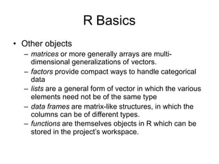
R is a language and environment for statistical computing and graphics. It includes facilities for data manipulation, calculation, graphical display, and programming. Some key features of R include effective data handling, a suite of operators for calculations on arrays and matrices, graphical facilities, and a programming language with conditionals, loops, and functions. Common data structures in R include vectors, matrices, factors, lists, and data frames. Basic operations include arithmetic, logical operations, indexing, subsetting, applying functions, binding, and coercing between different structures.

1. Introduction to R

2. R
• R is a language and environment for
statistical computing and graphics.
• Is open source
• http://www.r-project.org/

3. R
• R is an integrated suite of software facilities for data
manipulation, calculation and graphical display. It
includes
– an effective data handling and storage facility,
– a suite of operators for calculations on arrays, in particular
matrices,
– a large, coherent, integrated collection of intermediate tools for
data analysis,
– graphical facilities for data analysis and display either on-screen
or on hardcopy, and
– a well-developed, simple and effective programming language
which includes conditionals, loops, user-defined recursive
functions and input and output facilities.

4. The R Console

5. R basics
• From An Introduction to R (pdf guide) available
with the software
– Case sensitive
– Elementary commands – expressions (fancy
calculator) and assignments
– Commands separated by ; or newline
– All entities R creates and manipulates are known as
objects – command object() lists all current objects.
– All objects currently stored is the workspace
– To remove objects from workspace, rm(x, y, z)

6. R basics
• Simplest data structure in R is a vector
• x <- c(10.4, 5.6, 3.1, 6.4, 21.7)
– Assigns to x, the values contained in c()
– Can also use
• assign("x", c(10.4, 5.6, 3.1, 6.4, 21.7))
• c(10.4, 5.6, 3.1, 6.4, 21.7) -> x
• Can perform all arithmetic operations on these
vectors
• Arithmetic functions also available; so are min,
max, mean, sd, var, range etc.
• summary() provides – min, 1st qu, median,
mean, max etc.

7. R basics
• Logical vectors: TRUE or FALSE
– E.g. x == 10; temp <- x > 0
– <, >, <=, >=, ==, != are the operators
– x & y; x | y; !x
• Missing values
– Assigned special value NA
– is.na(x) gives a logical vector with value TRUE if and
only if the corresponding element in x is NA
– NaN ( 0 / 0) is also treated as missing value
– Can differentiate the two based on is.nan(x) function

8. R Basics
• Other objects
– matrices or more generally arrays are multi-
dimensional generalizations of vectors.
– factors provide compact ways to handle categorical
data
– lists are a general form of vector in which the various
elements need not be of the same type
– data frames are matrix-like structures, in which the
columns can be of different types.
– functions are themselves objects in R which can be
stored in the project’s workspace.

9. Exercise
• 2
• 2
• 2
• 2
• 2
• 1
• 1
• 3
• 2
• 1
2
1
2
4
1
3
3
2
4
1
• 3
• 1
• 2
• 3
• 2
• 2
• 3
• 2
• 2
• 2
4
3
3
2
3
2
2
1
4
2
# in HH # of trips # in HH # of trips
Create two variables nhh, ntrips with the above data points

10. Factor
• used to specify a discrete classification
(grouping) of the components of other vectors of
the same length
– nhhf <- factor(nhh)
– nhhf
– levels(nhhf)
– tripmeans <- tapply(ntrips, nhhf, mean)
– Create factor of ntrips;
– table(ntripsf, nhhf) gives?

11. Arrays
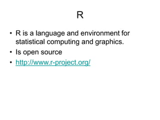
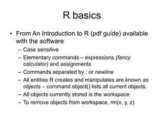
• A vector can be converted into an array
using the dim() function.
– dim(z) <- c(3,5,100)
– Index starts from 1,1,1
– Follows column major order – 1st subscript
incremented first; z[1,1,1], z[2,1,1]…
– Can also use array() function
• > x <- array(1:20, dim=c(4,5))
• > x

12. Matrix Operations
• Transpose: B <- t(A)
• nrow(A) and ncol(A)
• A * B – element by element multiplication
• A %*% B – matrix multiplication
• Can also use crossprod(X,y): same as t(X) %*% y
• diag()
– If argument is vector, a matrix with vector elements in diagonal is
returned
– If argument is matrix, diagonal elements returned as vector
– If argument is number k, a k by k Identity matrix is returned
• If you want to Invert matrices use, solve(A); if you want
to compute A-1x use solve(A,x)
• Matrix can be created using cbind() and rbind() too

13. Rbind
• df <- data.frame(a=c(1, 3, 3, 4, 5),
•
•
b=c(7, 7, 8, 3, 2),
c=c(3, 3, 6, 6, 8))
• #define vectors
• d <- c(11, 14, 16)
• e <- c(34, 35, 36)

14. • #rbind vectors to data frame
• df_new1 <- rbind(df, d, e)
• df_new2<- rbind(df, d)
• df_new3<- rbind(a,b)

15. • #create two data frames
• df1 <- data.frame(a=c(1, 3, 3, 4, 5),
• b=c(7, 7, 8, 3, 2),
• c=c(3, 3, 6, 6, 8))
• df2 <- data.frame(a=c(11, 14, 16, 17, 22),
• b=c(34, 35, 36, 36, 40),
• c=c(2, 2, 5, 7, 8))
• #rbind two data frames into one data frame
• df_new <- rbind(df1, df2)

16. Cbind
• #create two vectors
• a <- c(1, 3, 3, 4, 5)
• b <- c(7, 7, 8, 3, 2)
• #cbind the two vectors into a matrix
• new_matrix <- cbind(a, b)

17. • df <- data.frame(a=c(1, 3, 3, 4, 5),
•
•
b=c(7, 7, 8, 3, 2),
c=c(3, 3, 6, 6, 8))
• #define vector
• d <- c(11, 14, 16, 17, 22)
• #cbind vector to data frame
• df_new <- cbind(df, d)

18. Useful functions
• Sequences
– c(1,2,3,4,5) can be easily written as c(1:5) or
seq(1,5)
– seq(1,5,by=0.5) gives what?
– seq(from=1, by = 0.5, length = 10) gives
what?
• Repeating vectors
– temp <- rep(x, times = 5)
– temp<- rep(x, each =5)

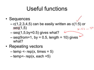
19. Useful functions
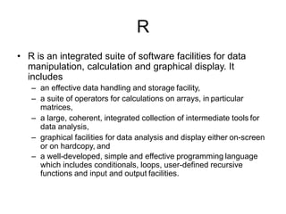
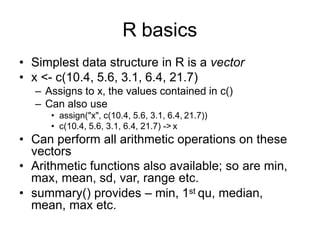
• Indexing Vectors
– Logical vector
• x <- c(1,2,4,NA,5)
• x[!is.na(x)] gives what?
• x[(!is.na(x)) & x > 2] gives what?
– Vector of positive integral quantities: x[1:3]
– Vector of –ve integral quantities: x[-(1:3)]
gives what?
• Replace all missing values in x with 0

20. Useful functions
• z <- 0:9; strz <- as.character(z); newz <-
as.integer(strz)
• truncate a vector: length(z) <- 3
• If you have a continuous variable, how will
you divide it into factors?
– cont <- rnorm(100, 50, 25)
– cont.fact <- cut(cont, 5)
– cont.fact2 <- cut(cont, 10+10*(0:9))