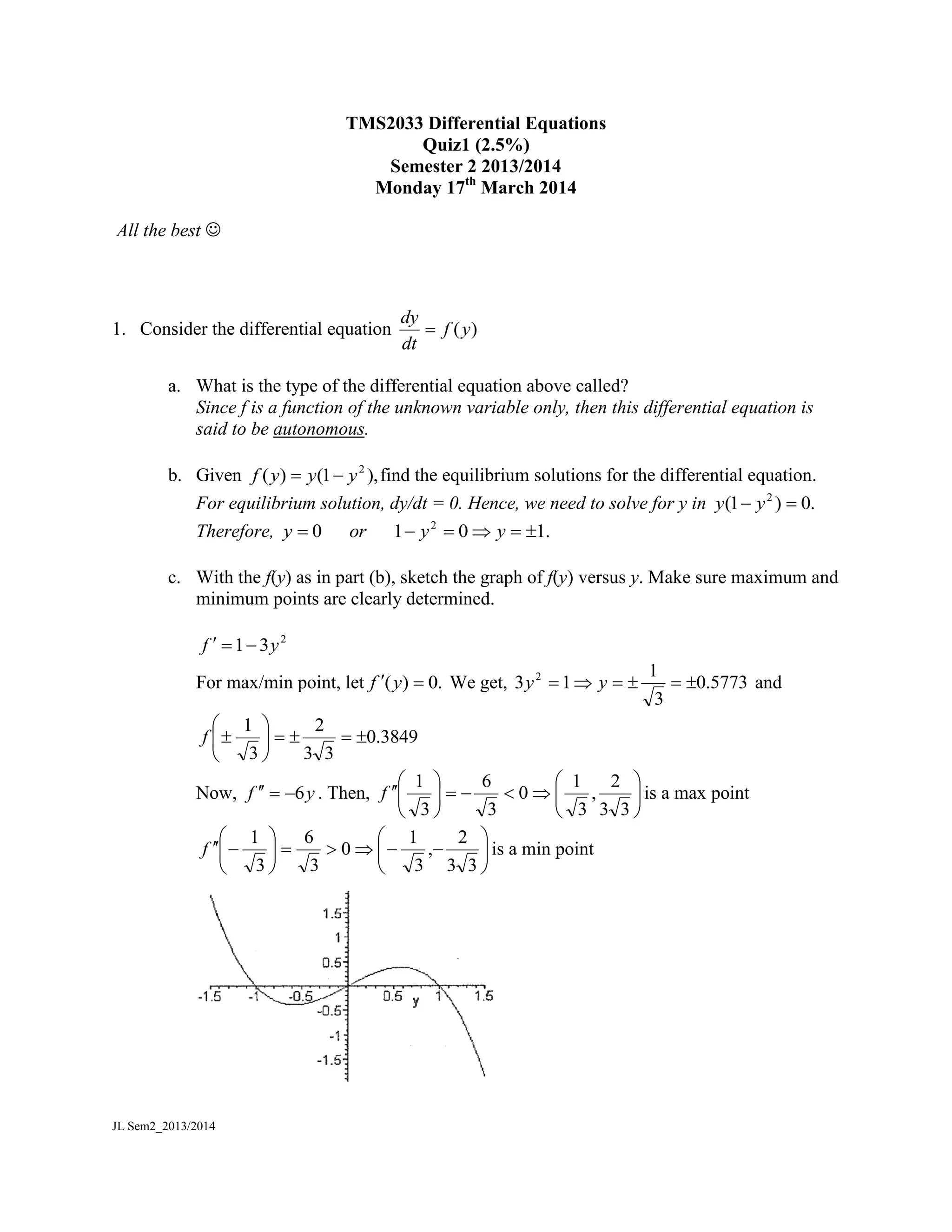
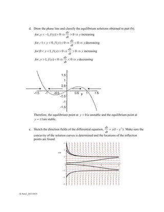
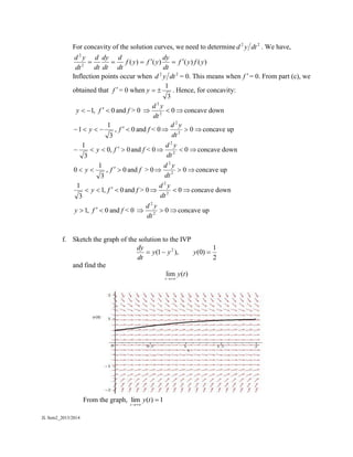
This document contains a quiz on differential equations with the following questions: 1) Find the equilibrium solutions and sketch the graph of an autonomous differential equation. 2) Draw the phase line and classify the equilibrium solutions. 3) Sketch the direction fields and find the inflection points and concavity of solution curves. 4) Graph the solution to an initial value problem and find its limit as t approaches infinity.

1. JL Sem2_2013/2014
TMS2033 Differential Equations
Quiz1 (2.5%)
Semester 2 2013/2014
Monday 17th
March 2014
All the best 
1. Consider the differential equation )(yf
dt
dy

a. What is the type of the differential equation above called?
Since f is a function of the unknown variable only, then this differential equation is
said to be autonomous.
b. Given ),1()( 2
yyyf  find the equilibrium solutions for the differential equation.
For equilibrium solution, dy/dt = 0. Hence, we need to solve for y in .0)1( 2
 yy
Therefore, .1010 2
 yyory
c. With the f(y) as in part (b), sketch the graph of f(y) versus y. Make sure maximum and
minimum points are clearly determined.
2
31 yf 
For max/min point, let .0)(  yf We get, 5773.0
3
1
13 2
 yy and
3849.0
33
2
3
1






f
Now, yf 6 . Then, 












33
2
,
3
1
0
3
6
3
1
f is a max point













33
2
,
3
1
0
3
6
3
1
f is a min point

2. JL Sem2_2013/2014
d. Draw the phase line and classify the equilibrium solutions obtained in part (b).
y
dt
dy
yfyfor  00)(,1, increasing
y
dt
dy
yfyfor  00)(,01, decreasing
y
dt
dy
yfyfor  00)(,10, increasing
y
dt
dy
yfyfor  00)(,1, decreasing
Therefore, the equilibrium point at 0y is unstable and the equilibrium point at
1y are stable.
e. Sketch the direction fields of the differential equation, ).1( 2
yy
dt
dy
 Make sure the
concavity of the solution curves is determined and the locations of the inflection
points are found.

3. JL Sem2_2013/2014
For concavity of the solution curves, we need to determine 22
dtyd . We have,
)()()()(2
2
yfyf
dt
dy
yfyf
dt
d
dt
dy
dt
d
dt
yd

Inflection points occur when 22
dtyd = 0. This means when f = 0. From part (c), we
obtained that f = 0 when
3
1
y . Hence, for concavity:
,1y 0f and f > 0  02
2
dt
yd
concave down
3
1
1  y , 0f and f < 0  02
2
dt
yd
concave up
0,0
3
1
 fy and f < 0  02
2
dt
yd
concave down
3
1
0  y , 0f and f > 0  02
2
dt
yd
concave up
0,1
3
1
 fy and f > 0  02
2
dt
yd
concave down
,1y 0f and f < 0  02
2
dt
yd
concave up
f. Sketch the graph of the solution to the IVP
2
1
)0(),1( 2
 yyy
dt
dy
and find the
lim ( )
t
y t

From the graph, 1)(lim 

ty
t