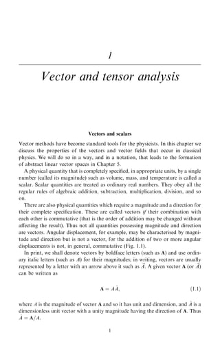
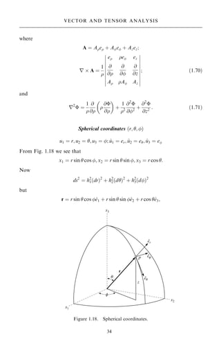
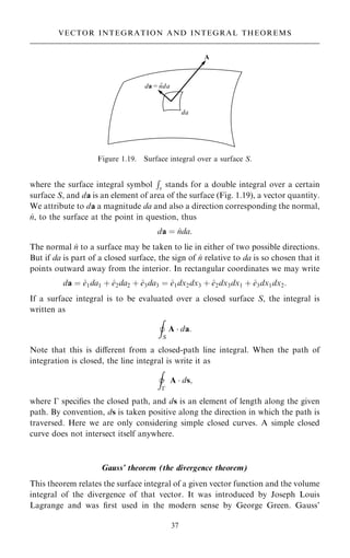
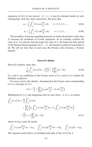
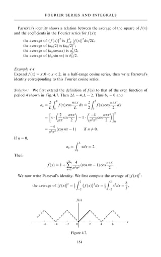
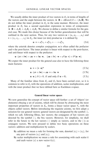
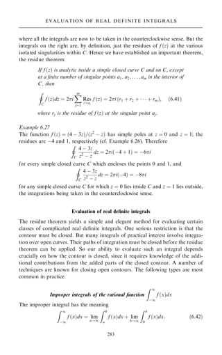
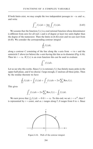
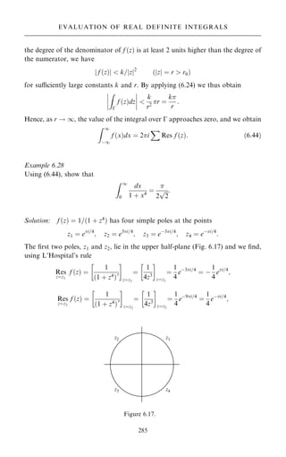
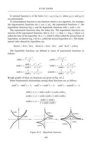
This document provides a summary of the book "Mathematical Methods for Physicists: A concise introduction" by Tai L. Chow. The book is designed as an intermediate-level textbook for a two-semester course in mathematical physics. It covers many of the core mathematical tools and concepts used in physics, including vector analysis, complex variables, linear algebra, Fourier analysis and special functions. The book aims to bridge the gap between introductory and more advanced physics courses. It contains many worked examples and exercises.
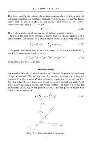
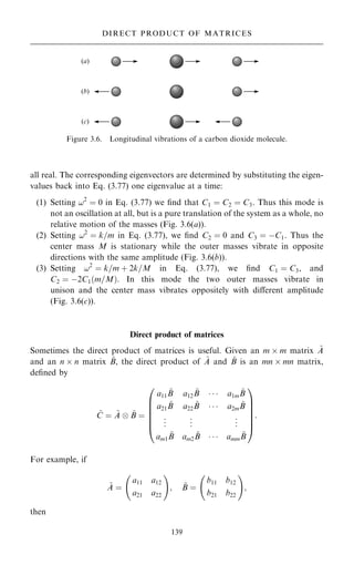
![will be introduced later. Consider the vector A expressed in terms of the unit
coordinate vectors …^
e1; ^
e2; ^
e3†:
A ˆ A1^
e1 ‡ A2^
e2 ‡ A^
e3 ˆ
X
3
iˆ1
Ai^
ei:
Relative to a new system …^
e0
1; ^
e0
2; ^
e0
3† that has a diÿerent orientation from that of
the old system …^
e1; ^
e2; ^
e3†, vector A is expressed as
A ˆ A0
1^
e0
1 ‡ A0
2^
e0
2 ‡ A0
^
e0
3 ˆ
X
3
iˆ1
A0
i ^
e0
i :
Note that the dot product A ^
e0
1 is equal to A0
1, the projection of A on the direction
of ^
e0
1; A ^
e0
2 is equal to A0
2, and A ^
e0
3 is equal to A0
3. Thus we may write
A0
1 ˆ …^
e1 ^
e0
1†A1 ‡ …^
e2 ^
e0
1†A2 ‡ …^
e3 ^
e0
1†A3;
A0
2 ˆ …^
e1 ^
e0
2†A1 ‡ …^
e2 ^
e0
2†A2 ‡ …^
e3 ^
e0
2†A3;
A0
3 ˆ …^
e1 ^
e0
3†A1 ‡ …^
e2 ^
e0
3†A2 ‡ …^
e3 ^
e0
3†A3:
9
=
;
…1:23†
The dot products …^
ei ^
e0
j † are the direction cosines of the axes of the new coordi-
nate system relative to the old system: ^
e0
i ^
ej ˆ cos…x0
i ; xj†; they are often called the
coecients of transformation. In matrix notation, we can write the above system
of equations as
A0
1
A0
2
A0
3
0
B
@
1
C
A ˆ
^
e1 ^
e0
1 ^
e2 ^
e0
1 ^
e3 ^
e0
1
^
e1 ^
e0
2 ^
e2 ^
e0
2 ^
e3 ^
e0
2
^
e1 ^
e0
3 ^
e2 ^
e0
3 ^
e3 ^
e0
3
0
B
@
1
C
A
A1
A2
A3
0
B
@
1
C
A:
The 3 3 matrix in the above equation is called the rotation (or transformation)
matrix, and is an orthogonal matrix. One advantage of using a matrix is that
successive transformations can be handled easily by means of matrix multiplica-
tion. Let us digress for a quick review of some basic matrix algebra. A full account
of matrix method is given in Chapter 3.
A matrix is an ordered array of scalars that obeys prescribed rules of addition
and multiplication. A particular matrix element is speci®ed by its row number
followed by its column number. Thus aij is the matrix element in the ith row and
jth column. Alternative ways of representing matrix ~
A are [aij] or the entire array
~
A ˆ
a11 a12 ::: a1n
a21 a22 ::: a2n
::: ::: ::: :::
am1 am2 ::: amn
0
B
B
B
B
@
1
C
C
C
C
A
:
12
VECTOR AND TENSOR ANALYSIS](https://image.slidesharecdn.com/mathematicalmethodsforphysicistschow-220911235848-a06d1992/85/Mathematical_Methods_for_Physicists_CHOW-pdf-27-320.jpg)
![(g) Is ~
A ÿ ~
AT
antisymmetric?
3.7 Show that the matrix
~
A ˆ
1 4 0
2 5 0
3 6 0
0
B
@
1
C
A
is not invertible.
3.8 Show that if ~
A and ~
B are invertible matrices of the same order, then ~
A ~
B is
invertible.
3.9 Given
~
A ˆ
1 2 3
2 5 3
1 0 8
0
B
@
1
C
A;
®nd ~
Aÿ1
and check the answer by direct multiplication.
3.10 Prove that if ~
A is a non-singular matrix, then det( ~
Aÿ1
† ˆ 1= det… ~
A).
3.11 If ~
A is an invertible n n matrix, show that ~
AX ˆ 0 has only the trivial
solution.
3.12 Show, by computing a matrix inverse, that the solution to the following
system is x1 ˆ 4, x2 ˆ 1:
x1 ÿ x2 ˆ 3;
x1 ‡ x2 ˆ 5:
3.13 Solve the system ~
AX ˆ ~
B if
~
A ˆ
1 0 0
0 2 0
0 0 1
0
B
@
1
C
A; ~
B ˆ
1
2
3
0
B
@
1
C
A:
3.14 Given matrix ~
A, ®nd A*, AT
, and Ay
, where
~
A ˆ
2 ‡ 3i 1 ÿ i 5i ÿ3
1 ‡ i 6 ÿ i 1 ‡ 3i ÿ1 ÿ 2i
5 ÿ 6i 3 0 ÿ4
0
B
@
1
C
A:
3.15 Show that:
(a) The matrix ~
A ~
Ay
, where ~
A is any matrix, is hermitian.
(b) … ~
A ~
B†y
ˆ ~
By ~
Ay
:
(c) If ~
A; ~
B are hermitian, then ~
A ~
B ‡ ~
B ~
A is hermitian.
(d) If ~
A and ~
B are hermitian, then i… ~
A ~
B ÿ ~
B ~
A† is hermitian.
3.16 Obtain the most general orthogonal matrix of order 2.
[Hint: use relations (3.34a) and (3.34b).]
3.17. Obtain the most general unitary matrix of order 2.
141
PROBLEMS](https://image.slidesharecdn.com/mathematicalmethodsforphysicistschow-220911235848-a06d1992/85/Mathematical_Methods_for_Physicists_CHOW-pdf-156-320.jpg)
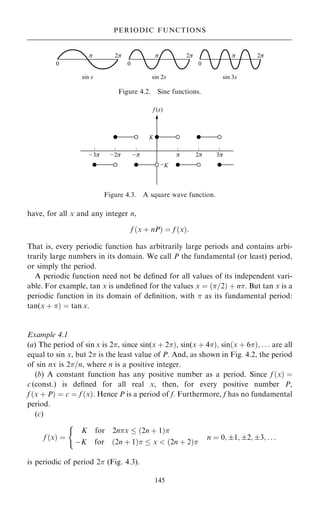
![Fourier series; Euler±Fourier formulas
If the general periodic function f …x† is de®ned in an interval ÿ x , the
Fourier series of f …x† in [ÿ; ] is de®ned to be a trigonometric series of the form
f …x† ˆ 1
2 a0 ‡ a1 cos x ‡ a2 cos 2x ‡ ‡ an cos nx ‡
‡ b1 sin x ‡ b2 sin 2x ‡ ‡ bn sin nx ‡ ; …4:2†
where the numbers a0; a1; a2; . . . ; b1; b2; b3; . . . are called the Fourier coecients of
f …x† in ‰ÿ; Š. If this expansion is possible, then our power to solve physical
problems is greatly increased, since the sine and cosine terms in the series can be
handled individually without diculty. Joseph Fourier (1768±1830), a French
mathematician, undertook the systematic study of such expansions. In 1807 he
submitted a paper (on heat conduction) to the Academy of Sciences in Paris and
claimed that every function de®ned on the closed interval ‰ÿ; Š could be repre-
sented in the form of a series given by Eq. (4.2); he also provided integral formulas
for the coecients an and bn. These integral formulas had been obtained earlier by
Clairaut in 1757 and by Euler in 1777. However, Fourier opened a new avenue by
claiming that these integral formulas are well de®ned even for very arbitrary
functions and that the resulting coecients are identical for diÿerent functions
that are de®ned within the interval. Fourier's paper was rejected by the Academy
on the grounds that it lacked mathematical rigor, because he did not examine the
question of the convergence of the series.
The trigonometric series (4.2) is the only series which corresponds to f …x†.
Questions concerning its convergence and, if it does, the conditions under
which it converges to f …x† are many and dicult. These problems were partially
answered by Peter Gustave Lejeune Dirichlet (German mathematician, 1805±
1859) and will be discussed brie¯y later.
Now let us assume that the series exists, converges, and may be integrated term
by term. Multiplying both sides by cos mx, then integrating the result from ÿ to
, we have
Z
ÿ
f …x† cos mx dx ˆ
a0
2
Z
ÿ
cos mx dx ‡
X
1
nˆ1
an
Z
ÿ
cos nx cos mx dx
‡
X
1
nˆ1
bn
Z
ÿ
sin nx cos mx dx: …4:3†
Now, using the following important properties of sines and cosines:
Z
ÿ
cos mx dx ˆ
Z
ÿ
sin mx dx ˆ 0 if m ˆ 1; 2; 3; . . . ;
Z
ÿ
cos mx cos nx dx ˆ
Z
ÿ
sin mx sin nx dx ˆ
0 if n 6ˆ m;
if n ˆ m;
(
146
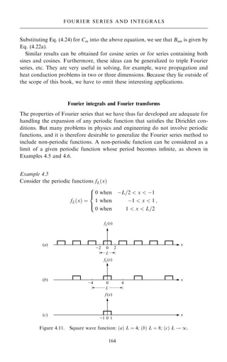
FOURIER SERIES AND INTEGRALS](https://image.slidesharecdn.com/mathematicalmethodsforphysicistschow-220911235848-a06d1992/85/Mathematical_Methods_for_Physicists_CHOW-pdf-161-320.jpg)
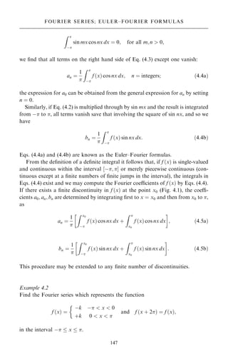
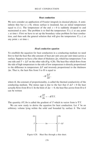
![Solution:
an ˆ
1
Z 0
ÿ
0 cos nt dt ‡
Z
0
sin t cos nt dt
ˆ ÿ
1
2
cos…1 ÿ n†t
1 ÿ n
‡
cos…1 ‡ n†t
1 ‡ n
0
ˆ
cos n ‡ 1
…1 ÿ n†2
; n 6ˆ 1
þ
þ
þ
þ
þ
;
a1 ˆ
1
Z
0
sin t cos t dt ˆ
1
sin2
t
2
þ
þ
þ
þ
0
ˆ 0;
bn ˆ
1
Z 0
ÿ
0 sin nt dt ‡
Z
0
sin t sin nt dt
ˆ
1
2
sin…1 ÿ n†t
1 ÿ n
ÿ
sin…1 ‡ n†t
1 ‡ n
0
ˆ 0
b1 ˆ
1
Z
0
sin2
t dt ˆ
1
t
2
ÿ
sin 2t
4
0
ˆ
1
2
:
Accordingly the Fourier expansion of f …t† in [ÿ; ] may be written
f …t† ˆ
1
‡
sin t
2
ÿ
2
cos 2t
3
‡
cos 4t
15
‡
cos 6t
35
‡
cos 8t
63
‡
:
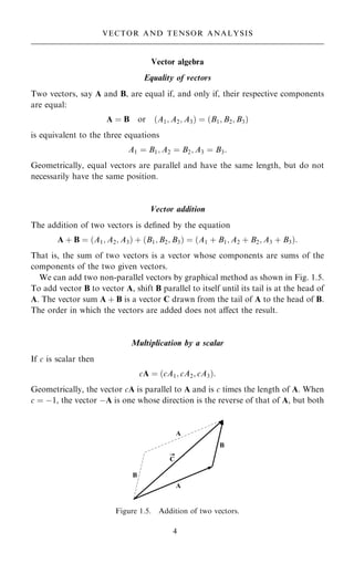
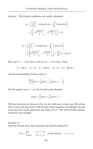
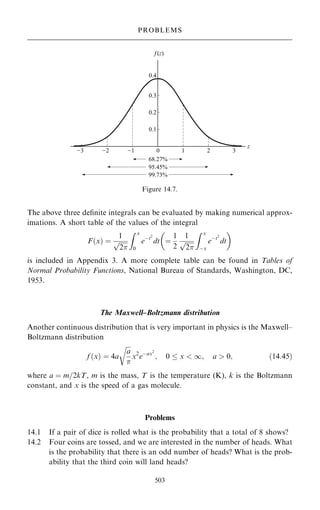
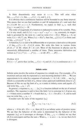
The ®rst three partial sums Sn…n ˆ 1; 2; 3) are shown in Fig. 4.5: S1 ˆ 1=;
S2 ˆ 1= ‡ sin t=2, and S3 ˆ 1= ‡ sin …t†=2 ÿ 2 cos …2t†=3:
149
FOURIER SERIES; EULER±FOURIER FORMULAS
Figure 4.4. The ®rst two partial sums.](https://image.slidesharecdn.com/mathematicalmethodsforphysicistschow-220911235848-a06d1992/85/Mathematical_Methods_for_Physicists_CHOW-pdf-164-320.jpg)

![In general A
~
B
~
6ˆ B
~
A
~
. The diÿerence A
~
B
~
ÿB
~
A
~
is called the commutator of A
~
and B
~
and is denoted by the symbol ‰A
~
; B
~
]:
‰A
~
; B
~
Š A
~
B
~
ÿB
~
A
~
: …5:18†
An operator whose commutator vanishes is called a commuting operator.
The operator equation
B
~
ˆ A
~
ˆ A
~
is equivalent to the vector equation
B
~
j i ˆ A
~
j i for any j i:
And the vector equation
A
~
j i ˆ j i
is equivalent to the operator equation
A
~
ˆ E
~
where E
~
is the identity (or unit) operator:
E
~
j i ˆ j i for any j i:
It is obvious that the equation A
~
ˆ is meaningless.
Example 5.11
To illustrate the non-commuting nature of operators, let A
~
ˆ x; B
~
ˆ d=dx. Then
A
~
B
~
f …x† ˆ x
d
dx
f …x†;
and
B
~
A
~
f …x† ˆ
d
dx
xf …x† ˆ
dx
dx
f ‡ x
df
dx
ˆ f ‡ x
df
dx
ˆ …E
~
‡A
~
B
~
† f :
Thus,
…A
~
B
~
ÿB
~
A
~
† f …x† ˆ ÿE
~
f …x†
or
x;
d
dx
ˆ x
d
dx
ÿ
d
dx
x ˆ ÿE
~
:
Having de®ned the product of two operators, we can also de®ne an operator
raised to a certain power. For example
A
~
m
j i ˆ A
~
A
~
A
~
j i:
216
LINEAR VECTOR SPACES
|‚‚‚‚‚‚‚‚‚‚‚‚‚{z‚‚‚‚‚‚‚‚‚‚‚‚‚}
m factor](https://image.slidesharecdn.com/mathematicalmethodsforphysicistschow-220911235848-a06d1992/85/Mathematical_Methods_for_Physicists_CHOW-pdf-231-320.jpg)


![By setting q ˆ …z ÿ a†=…w ÿ a† we ®nd
1
1 ÿ ‰…z ÿ a†=…w ÿ a†Š
ˆ 1 ‡
z ÿ a
w ÿ a
‡
z ÿ a
w ÿ a
2
‡ ‡
z ÿ a
w ÿ a
n
‡
‰…z ÿ a†=…w ÿ a†Šn‡1
…w ÿ z†=…w ÿ a†
:
We insert this into Eq. (6.33). Since z and a are constant, we may take the powers
of (z ÿ a) out from under the integral sign, and then Eq. (6.33) takes the form
f …z† ˆ
1
2i
I
C
f …w†dw
w ÿ a
‡
z ÿ a
2i
I
C
f …w†dw
…w ÿ a†2
‡ ‡
…z ÿ a†n
2i
I
C
f …w†dw
…w ÿ a†n‡1
‡ Rn…z†:
Using Eq. (6.28), we may write this expansion in the form
f …z† ˆ f …a† ‡
z ÿ a
1!
f 0
…a† ‡
…z ÿ a†2
2!
f 00
…a† ‡ ‡
…z ÿ a†n
n!
f n
…a† ‡ Rn…z†;
where
Rn…z† ˆ …z ÿ a†n 1
2i
I
C
f …w†dw
…w ÿ a†n
…w ÿ z†
:
Clearly, the expansion will converge and represent f …z† if and only if
limn!1 Rn…z† ˆ 0. This is easy to prove. Note that w is on C while z is inside
C, so we have jw ÿ zj 0. Now f …z† is analytic inside C and on C, so it follows
that the absolute value of f …w†=…w ÿ z† is bounded, say,
f …w†
w ÿ z
ÿ
ÿ
ÿ
ÿ
ÿ
ÿ
ÿ
ÿ M
for all w on C. Let r be the radius of C, then jw ÿ aj ˆ r for all w on C, and C has
the length 2r. Hence we obtain
Rn
j j ˆ
jz ÿ ajn
2
I
C
f …w†dw
…w ÿ a†n
…w ÿ z†
ÿ
ÿ
ÿ
ÿ
ÿ
ÿ
ÿ
ÿ
z ÿ a
j jn
2
M
1
rn 2r
ˆ Mr
z ÿ a
r
ÿ
ÿ
ÿ
ÿ
ÿ
ÿ
n
! 0 as n ! 1:
Thus
f …z† ˆ f …a† ‡
z ÿ a
1!
f 0
…a† ‡
…z ÿ a†2
2!
f 00
…a† ‡ ‡
…z ÿ a†n
n!
f n
…a†
is a valid representation of f …z† at all points in the interior of any circle with its
center at a and within which f …z† is analytic. This is called the Taylor series of f …z†
with center at a. And the particular case where a ˆ 0 is called the Maclaurin series
of f …z† [Colin Maclaurin 1698±1746, Scots mathematician].
271
SERIES REPRESENTATIONS OF ANALYTIC FUNCTIONS](https://image.slidesharecdn.com/mathematicalmethodsforphysicistschow-220911235848-a06d1992/85/Mathematical_Methods_for_Physicists_CHOW-pdf-286-320.jpg)
![Example 6.21
Expand ln(a ‡ z) about a.
Solution: Suppose we know the Maclaurin series, then
ln…1 ‡ z†ˆln…1 ‡ a ‡ z ÿ a† ˆ ln…1 ‡ a† 1 ‡
z ÿ a
1 ‡ a
ˆ ln…1 ‡ a† ‡ ln 1 ‡
z ÿ a
1 ‡ a
ˆln…1 ‡ a† ‡
z ÿ a
1 ‡ a
ÿ
1
2
z ÿ a
1 ‡ a
2
‡
1
3
z ÿ a
1 ‡ a
3
ÿ ‡ :
Example 6.22
Let f …z† ˆ ln…1 ‡ z†, and consider that branch which has the value zero when
z ˆ 0.
(a) Expand f …z† in a Taylor series about z ˆ 0, and determine the region of
convergence.
(b) Expand ln[(1 ‡ z†=…1 ÿ z)] in a Taylor series about z ˆ 0.
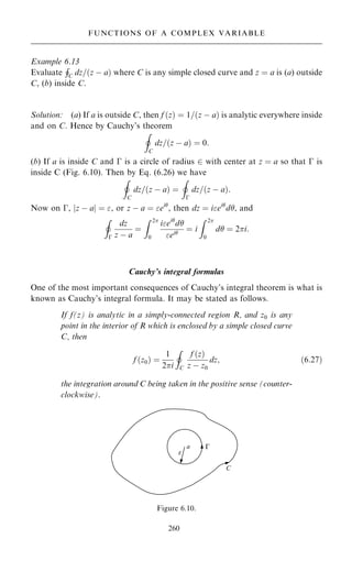
Solution: (a)
f …z† ˆ ln…1 ‡ z† f …0† ˆ 0
f 0
…z† ˆ …1 ‡ z†ÿ1
f 0
…0† ˆ 1
f 00
…z† ˆ ÿ…1 ‡ z†ÿ2
f 00
…0† ˆ ÿ1
f F…z† ˆ 2…1 ‡ z†ÿ3
f F…0† ˆ 2!
.
.
. .
.
.
f …n‡1†
…z† ˆ …ÿ1†n
n!…1 ‡ n†…n‡1†
f …n‡1†
…0† ˆ …ÿ1†n
n!:
Then
f …z† ˆ ln…1 ‡ z† ˆ f …0† ‡ f 0
…0†z ‡
f 00
…0†
2!
z2
‡
f F…0†
3!
z3
‡
ˆ z ÿ
z2
2
‡
z3
3
ÿ
z4
4
‡ ÿ :
The nth term is un ˆ …ÿ1†nÿ1
zn
=n. The ratio test gives
lim
n!1
un‡1
un
ÿ
ÿ
ÿ
ÿ
ÿ
ÿ
ÿ
ÿ ˆ lim
n!1
nz
n ‡ 1
ÿ
ÿ
ÿ
ÿ
ÿ
ÿ
ÿ
ÿ ˆ z
j j
and the series converges for jzj 1.
273
SERIES REPRESENTATIONS OF ANALYTIC FUNCTIONS](https://image.slidesharecdn.com/mathematicalmethodsforphysicistschow-220911235848-a06d1992/85/Mathematical_Methods_for_Physicists_CHOW-pdf-288-320.jpg)
![Substituting this and its derivatives into Eq. (7.1) and denoting the constant
… ‡ 1† by k we obtain
…1 ÿ x2
†
X
1
mˆ2
m…m ÿ 1†amxmÿ2
ÿ 2x
X
1
mˆ1
mamxmÿ1
‡ k
X
1
mˆ0
amxm
ˆ 0:
By writing the ®rst term as two separate series we have
X
1
mˆ2
m…m ÿ 1†amxmÿ2
ÿ
X
1
mˆ2
m…m ÿ 1†amxm
ÿ 2
X
1
mˆ1
mamxm
‡ k
X
1
mˆ0
amxm
ˆ 0;
which can be written as:
2 1a2 ‡ 3 2a3x ‡ 4 3a4x2
‡ ‡ …s ‡ 2†…s ‡ 1†as‡2xs
‡
ÿ2 1a2x2
ÿ ÿ …s…s ÿ 1†asxs
ÿ
ÿ2 1a1x ÿ 2 2a2x2
ÿ ÿ 2sasxs
ÿ
‡ka0 ‡ ka1x ‡ ka2x2
‡ ‡ kasxs
‡ ˆ 0:
Since this must be an identity in x if Eq. (7.2) is to be a solution of Eq. (7.1), the
sum of the coecients of each power of x must be zero; remembering that
k ˆ … ‡ 1† we thus have
2a2 ‡ … ‡ 1†a0 ˆ 0; …7:3a†
6a3 ‡ ‰ÿ2 ‡ v…v ‡ 1†Ša1 ˆ 0; …7:3b†
and in general, when s ˆ 2; 3; . . . ;
…s ‡ 2†…s ‡ 1†as‡2 ‡ ‰ÿs…s ÿ 1† ÿ 2s ‡ …‡1†Šas ˆ 0: …4:4†
The expression in square brackets [. . .] can be written
… ÿ s†… ‡ s ‡ 1†:
We thus obtain from Eq. (7.4)
as‡2 ˆ ÿ
… ÿ s†… ‡ s ‡ 1†
…s ‡ 2†…s ‡ 1†
as …s ˆ 0; 1; . . .†: …7:5†
This is a recursion formula, giving each coecient in terms of the one two places
before it in the series, except for a0 and a1, which are left as arbitrary constants.
297
LEGENDRE'S EQUATION](https://image.slidesharecdn.com/mathematicalmethodsforphysicistschow-220911235848-a06d1992/85/Mathematical_Methods_for_Physicists_CHOW-pdf-312-320.jpg)

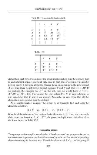
![The same set of all integers does not form a group under multiplication. Why?
Because the inverses of integers are not integers and so they are not members of
the set.
Example 12.3
The set of all rational numbers (p=q, with q 6ˆ 0) forms a continuous in®nite group
under addition. It is an Abelian group, and we denote it by S2. The identity
element is 0; and the inverse of a given element is its negative.
Example 12.4
The set of all complex numbers …z ˆ x ‡ iy† forms an in®nite group under
addition. It is an Abelian group and we denote it by S3. The identity element
is 0; and the inverse of a given element is its negative (that is, ÿz is the inverse
of z).
The set of elements in S1 is a subset of elements in S2, and the set of elements in
S2 is a subset of elements in S3. Furthermore, each of these sets forms a group
under addition, thus S1 is a subgroup of S2, and S2 a subgroup of S3. Obviously
S1 is also a subgroup of S3.
Example 12.5
The three matrices
~
A ˆ
1 0
0 1
; ~
B ˆ
0 1
ÿ1 ÿ1
; ~
C ˆ
ÿ1 ÿ1
1 0
form an Abelian group of order three under matrix multiplication. The identity
element is the unit matrix, E ˆ ~
A. The inverse of a given matrix is the inverse
matrix of the given matrix:
~
Aÿ1
ˆ
1 0
0 1
ˆ ~
A; ~
Bÿ1
ˆ
ÿ1 ÿ1
1 0
ˆ ~
C; ~
Cÿ1
ˆ
0 1
ÿ1 ÿ1
ˆ ~
B:
It is straightforward to check that all the four group axioms are satis®ed. We
leave this to the reader.
Example 12.6
The three permutation operations on three objects a; b; c
‰1 2 3Š; ‰2 3 1Š; ‰3 1 2Š
form an Abelian group of order three with sequential performance as the law of
combination.
The operation [1 2 3] means we put the object a ®rst, object b second, and object
c third. And two elements are multiplied by performing ®rst the operation on the
432
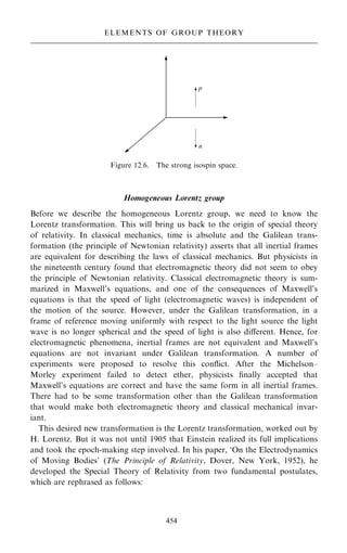
ELEMENTS OF GROUP THEORY](https://image.slidesharecdn.com/mathematicalmethodsforphysicistschow-220911235848-a06d1992/85/Mathematical_Methods_for_Physicists_CHOW-pdf-447-320.jpg)
![right, then the operation on the left. For example
‰2 3 1Š‰3 1 2Šabc ˆ ‰2 3 1Šcab ˆ abc:
Thus two operations performed sequentially are equivalent to the operation
[1 2 3]:
‰2 3 1Š‰3 1 2Š ˆ ‰1 2 3Š:
similarly
‰3 1 2Š‰2 3 1Šabc ˆ ‰3 1 2Šbca ˆ abc;
that is,
‰3 1 2Š‰2 3 1Š ˆ ‰1 2 3Š:
This law of combination is commutative. What is the identity element of this
group? And the inverse of a given element? We leave the reader to answer these
questions. The group illustrated by this example is known as a cyclic group of
order 3, C3.
It can be shown that the set of all permutations of three objects
‰1 2 3Š; ‰2 3 1Š; ‰3 1 2Š; ‰1 3 2Š; ‰3 2 1Š; ‰2 1 3Š
forms a non-Abelian group of order six denoted by S3. It is called the symmetric
group of three objects. Note that C3 is a subgroup of S3.
Cyclic groups
We now revisit the cyclic groups. The elements of a cyclic group can be expressed
as power of a single element A, say, as A; A2
; A3
; . . . ; Apÿ1
; Ap
ˆ E; p is the smal-
lest integer for which Ap
ˆ E and is the order of the group. The inverse of Ak
is
Apÿk
, that is, an element of the set. It is straightforward to check that all group
axioms are satis®ed. We leave this to the reader. It is obvious that cyclic groups
are Abelian since Ak
A ˆ AAk
…k p†.
Example 12.7
The complex numbers 1, i; ÿ1; ÿi form a cyclic group of order 3. In this case,
A ˆ i and p ˆ 3: in
, n ˆ 0; 1; 2; 3. These group elements may be interpreted as
successive 908 rotations in the complex plane …0; =2; ; and 3=2†. Con-
sequently, they can be represented by four 2 2 matrices. We shall come back
to this later.
Example 12.8
We now consider a second example of cyclic groups: the group of rotations of an
equilateral triangle in its plane about an axis passing through its center that brings
433
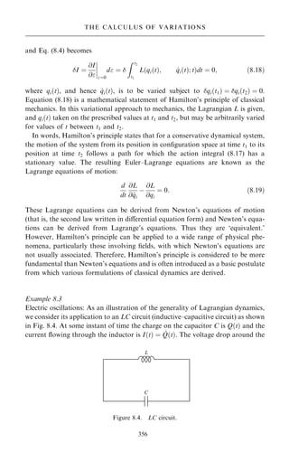
CYCLIC GROUPS](https://image.slidesharecdn.com/mathematicalmethodsforphysicistschow-220911235848-a06d1992/85/Mathematical_Methods_for_Physicists_CHOW-pdf-448-320.jpg)
![where yi ˆ f …xi†; yz ˆ f …z†. Or
i…z† ˆ
Z z
xi
f …x†dx ÿ
h
2
‰ f …xi† ÿ f …z†Š
ˆ
Z z
xi
f …x†dx ÿ
z ÿ xi
2
‰ f …xi† ÿ f …z†Š:
Diÿerentiating with respect to z:
0
i …z† ˆ f …z† ÿ ‰ f …xi† ‡ f …z†Š=2 ÿ …z ÿ xi† f 0
…z†=2:
Diÿerentiating once again,
00
i …z† ˆ ÿ…z ÿ xi†f 00
…z†=2:
If mi and Mi are, respectively, the minimum and the maximum values of f 00
…z† in
the subinterval [xi; z], we can write
z ÿ xi
2
mi ÿ00
i …z†
z ÿ xi
2
Mi:
Anti-diÿerentiation gives
…z ÿ xi†2
4
mi ÿ0
i …z†
…z ÿ xi†2
4
Mi
Anti-diÿerentiation once more gives
…z ÿ xi†3
12
mi ÿi…z†
…z ÿ xi†3
12
Mi:
or, since z ÿ xi ˆ h,
h3
12
mi ÿi
h3
12
Mi:
If m and M are, respectively, the minimum and the maximum of f 00
…z† in the
interval [a; b] then
h3
12
m ÿi
h3
12
M for all i:
Adding the errors for all subintervals, we obtain
h3
12
nm ÿ
h3
12
nM
or, since h ˆ …b ÿ a†=n;
…b ÿ a†3
12n2
m ÿ
…b ÿ a†3
12n2
M: …13:16†
468
NUMERICAL METHODS](https://image.slidesharecdn.com/mathematicalmethodsforphysicistschow-220911235848-a06d1992/85/Mathematical_Methods_for_Physicists_CHOW-pdf-483-320.jpg)

![Problem A1.13
Test for convergence the series
1
2
2
‡
1 3
2 4
2
‡
1 3 5
2 4 6
2
‡ ‡
1 3 5 …2n ÿ 1†
1 3 5 …2n†
‡ :
Hint: Neither the ratio test nor Raabe's test is applicable (show this). Try Gauss'
test.
Series of functions and uniform convergence
The series considered so far had the feature that un depended just on n. Thus the
series, if convergent, is represented by just a number. We now consider series
whose terms are functions of x; un ˆ un…x†. There are many such series of func-
tions. The reader should be familiar with the power series in which the nth term is
a constant times xn
:
S…x† ˆ
X
1
nˆ0
anxn
: …A1:4†
We can think of all previous cases as power series restricted to x ˆ 1. In later
sections we shall see Fourier series whose terms involve sines and cosines, and
other series in which the terms may be polynomials or other functions. In this
section we consider power series in x.
The convergence or divergence of a series of functions depends, in general, on
the values of x. With x in place, the partial sum Eq. (A1.2) now becomes a
function of the variable x:
sn…x† ˆ u1 ‡ u2…x† ‡ ‡ un…x†: …A1:5†
as does the series sum. If we de®ne S…x† as the limit of the partial sum
S…x† ˆ lim
n!1
sn…x† ˆ
X
1
nˆ0
un…x†; …A1:6†
then the series is said to be convergent in the interval [a, b] (that is, a x b), if
for each 0 and each x in [a, b] we can ®nd N 0 such that
S…x† ÿ sn…x†
j j ; for all n N: …A1:7†
If N depends only on and not on x, the series is called uniformly convergent in
the interval [a, b]. This says that for our series to be uniformly convergent, it must
be possible to ®nd a ®nite N so that the remainder of the series after N terms,
P1
iˆN‡1 ui…x†, will be less than an arbitrarily small for all x in the given interval.
The domain of convergence (absolute or uniform) of a series is the set of values
of x for which the series of functions converges (absolutely or uniformly).
520
APPENDIX 1 PRELIMINARIES](https://image.slidesharecdn.com/mathematicalmethodsforphysicistschow-220911235848-a06d1992/85/Mathematical_Methods_for_Physicists_CHOW-pdf-535-320.jpg)
![We deal with power series in x exactly as before. For example, we can use the
ratio test, which now depends on x, to investigate convergence or divergence of a
series:
r…x† ˆ lim
n!1
un‡1
un
þ
þ
þ
þ
þ
þ
þ
þ ˆ lim
n!1
þ
þ
þ
þ
an‡1xn‡1
anxn
þ
þ
þ
þ ˆ x
j j lim
n!1
an‡1
an
þ
þ
þ
þ
þ
þ
þ
þ ˆ x
j jr; r ˆ lim
n!1
an‡1
an
þ
þ
þ
þ
þ
þ
þ
þ;
thus the series converges (absolutely) if jxjr 1 or
jxj R ˆ
1
r
ˆ lim
n!1
an
an‡1
þ
þ
þ
þ
þ
þ
þ
þ
and the domain of convergence is given by R : ÿR x R. Of course, we need to
modify the above discussion somewhat if the power series does not contain every
power of x.
Example A1.13
For what value of x does the series
P1
nˆ1 xnÿ1
=n 3n
converge?
Solution: Now un ˆ xnÿ1
=n 3n
, and x 6ˆ 0 (if x ˆ 0 the series converges). We
have
lim
n!1
un‡1
un
þ
þ
þ
þ
þ
þ
þ
þ ˆ lim
n!1
n
3…n ‡ 1†
x
j j ˆ
1
3
x
j j:
Then the series converges if jxj 3, and diverges if jxj 3. If jxj ˆ 3, that is,
x ˆ 3, the test fails.
If x ˆ 3, the series becomes
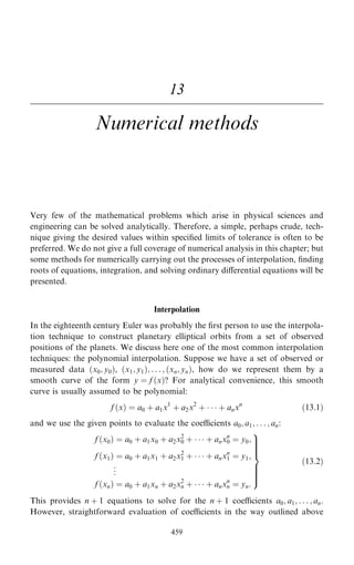
P1
nˆ1 1=3n which diverges. If x ˆ ÿ3, the series
becomes
P1
nˆ1…ÿ1†nÿ1
=3n which converges. Then the interval of convergence is
ÿ3 x 3. The series diverges outside this interval. Furthermore, the series
converges absolutely for ÿ3 x 3 and converges conditionally at x ˆ ÿ3.
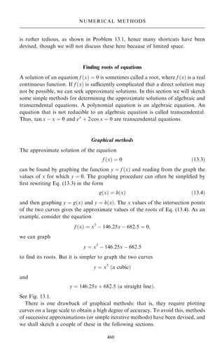
As for uniform convergence, the most commonly encountered test is the
Weierstrass M test:
Weierstrass M test
If a sequence of positive constants M1; M2; M3; . . . ; can be found such that: (a)
Mn jun…x†j for all x in some interval [a, b], and (b)
P
Mn converges, then
P
un…x† is uniformly and absolutely convergent in [a, b].
The proof of this common test is direct and simple. Since
P
Mn converges,
some number N exists such that for n N,
X
1
iˆN‡1
Mi :
521
SERIES OF FUNCTIONS AND UNIFORM CONVERGENCE](https://image.slidesharecdn.com/mathematicalmethodsforphysicistschow-220911235848-a06d1992/85/Mathematical_Methods_for_Physicists_CHOW-pdf-536-320.jpg)
![This follows from the de®nition of convergence. Then, with Mn jun…x†j for all x
in [a, b],
X
1
iˆN‡1
ui…x†
j j :
Hence
S…x† ÿ sn…x†
j j ˆ
þ
þ
þ
þ
X
1
iˆN‡1
ui…x†
þ
þ
þ
þ ; for all n N
and by de®nition
P
un…x† is uniformly convergent in [a, b]. Furthermore, since we
have speci®ed absolute values in the statement of the Weierstrass M test, the series
P
un…x† is also seen to be absolutely convergent.
It should be noted that the Weierstrass M test only provides a sucient con-
dition for uniform convergence. A series may be uniformly convergent even when
the M test is not applicable. The Weierstrass M test might mislead the reader to
believe that a uniformly convergent series must be also absolutely convergent, and
conversely. In fact, the uniform convergence and absolute convergence are inde-
pendent properties. Neither implies the other.
A somewhat more delicate test for uniform convergence that is especially useful
in analyzing power series is Abel's test. We now state it without proof.
Abel's test
If …a† un…x† ˆ an fn…x†, and
P
an ˆ A, convergent, and (b) the functions fn…x† are
monotonic ‰ fn‡1…x† fn…x†Š and bounded, 0 fn…x† M for all x in [a, b], then
P
un…x† converges uniformly in [a, b].
Example A1.14
Use the Weierstrass M test to investigate the uniform convergence of
…a†
X
1
nˆ1
cos nx
n4
; …b†
X
1
nˆ1
xn
n3=2
; …c†
X
1
nˆ1
sin nx
n
:
Solution:
(a) cos…nx†=n4
þ
þ
þ
þ 1=n4
ˆ Mn. Then since
P
Mn converges (p series with
p ˆ 4 1), the series is uniformly and absolutely convergent for all x by
the M test.
(b) By the ratio test, the series converges in the interval ÿ1 x 1 (or jxj 1).
For all x in jxj 1; xn
=n3=2
þ
þ
þ
þ
þ
þ ˆ x
j jn
=n3=2
1=n3=2
. Choosing Mn ˆ 1=n3=2
,
we see that
P
Mn converges. So the given series converges uniformly for
jxj 1 by the M test.
522
APPENDIX 1 PRELIMINARIES](https://image.slidesharecdn.com/mathematicalmethodsforphysicistschow-220911235848-a06d1992/85/Mathematical_Methods_for_Physicists_CHOW-pdf-537-320.jpg)
![(c) sin…nx†=n=n
j j 1=n ˆ Mn. However,
P
Mn does not converge. The M test
cannot be used in this case and we cannot conclude anything about the
uniform convergence by this test.
A uniformly convergent in®nite series of functions has many of the properties
possessed by the sum of ®nite series of functions. The following three are parti-
cularly useful. We state them without proofs.
(1) If the individual terms un…x† are continuous in [a, b] and if
P
un…x† con-
verges uniformly to the sum S…x† in [a, b], then S…x† is continuous in [a, b].
Brie¯y, this states that a uniformly convergent series of continuous func-
tions is a continuous function.
(2) If the individual terms un…x† are continuous in [a, b] and if
P
un…x† con-
verges uniformly to the sum S…x† in [a, b], then
Z b
a
S…x†dx ˆ
X
1
nˆ1
Z b
a
un…x†dx
or
Z b
a
X
1
nˆ1
un…x†dx ˆ
X
1
nˆ1
Z b
a
un…x†dx:
Brie¯y, a uniform convergent series of continuous functions can be inte-
grated term by term.
(3) If the individual terms un…x† are continuous and have continuous derivatives
in [a, b] and if
P
un…x† converges uniformly to the sum S…x† while
P
dun…x†=dx is uniformly convergent in [a, b], then the derivative of the
series sum S…x† equals the sum of the individual term derivatives,
d
dx
S…x† ˆ
X
1
nˆ1
d
dx
un…x† or
d
dx
X
1
nˆ1
un…x†
( )
ˆ
X
1
nˆ1
d
dx
un…x†:
Term-by-term integration of a uniformly convergent series requires only con-
tinuity of the individual terms. This condition is almost always met in physical
applications. Term-by-term integration may also be valid in the absence of uni-
form convergence. On the other hand term-by-term diÿerentiation of a series is
often not valid because more restrictive conditions must be satis®ed.
Problem A1.14
Show that the series
sin x
13
‡
sin 2x
23
‡ ‡
sin nx
n3
‡
is uniformly convergent for ÿ x .
523
SERIES OF FUNCTIONS AND UNIFORM CONVERGENCE](https://image.slidesharecdn.com/mathematicalmethodsforphysicistschow-220911235848-a06d1992/85/Mathematical_Methods_for_Physicists_CHOW-pdf-538-320.jpg)
![Theorems on power series
When we are working with power series and the functions they represent, it is very
useful to know the following theorems which we will state without proof. We will
see that, within their interval of convergence, power series can be handled much
like polynomials.
(1) A power series converges uniformly and absolutely in any interval which lies
entirely within its interval of convergence.
(2) A power series can be diÿerentiated or integrated term by term over any
interval lying entirely within the interval of convergence. Also, the sum of a
convergent power series is continuous in any interval lying entirely within its
interval of convergence.
(3) Two power series can be added or subtracted term by term for each value of
x common to their intervals of convergence.
(4) Two power series, for example,
P1
nˆ0 anxn
and
P1
nˆ0 bnxn
, can be multiplied
to obtain
P1
nˆ0 cnxn
; where cn ˆ a0bn ‡ a1bnÿ1 ‡ a2bnÿ2 ‡ ‡ anb0, the
result being, valid for each x within the common interval of convergence.
(5) If the power series
P1
nˆ0 anxn
is divided by the power series
P1
nˆ0 bnxn
,
where b0 6ˆ 0, the quotient can be written as a power series which converges
for suciently small values of x.
Taylor's expansion
It is very useful in most applied work to ®nd power series that represent the given
functions. We now review one method of obtaining such series, the Taylor expan-
sion. We assume that our function f …x† has a continuous nth derivative in the
interval [a, b] and that there is a Taylor series for f …x† of the form
f …x† ˆ a0 ‡ a1…x ÿ † ‡ a2…x ÿ †2
‡ a3…x ÿ †3
‡ ‡ an…x ÿ †n
‡ ;
…A1:8†
where lies in the interval [a, b]. Diÿerentiating, we have
f 0
…x† ˆ a1 ‡ 2a2…x ÿ † ‡ 3a3…x ÿ †2
‡ ‡ nan…x ÿ †nÿ1
‡ ;
f 00
…x† ˆ 2a2 ‡ 3 2a3…x ÿ † ‡ 4 3a4…x ÿ a†2
‡ ‡ n…n ÿ 1†an…x ÿ †nÿ2
‡ ;
.
.
.
f …n†
…x† ˆ n…n ÿ 1†…n ÿ 2† 1 an ‡ terms containing powers of …x ÿ †:
We now put x ˆ in each of the above derivatives and obtain
f …† ˆ a0; f 0
…† ˆ a1; f 00
…† ˆ 2a2; f F…† ˆ 3!a3; ; f …n†
…† ˆ n!an;
524
APPENDIX 1 PRELIMINARIES](https://image.slidesharecdn.com/mathematicalmethodsforphysicistschow-220911235848-a06d1992/85/Mathematical_Methods_for_Physicists_CHOW-pdf-539-320.jpg)
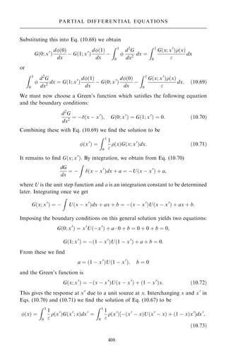
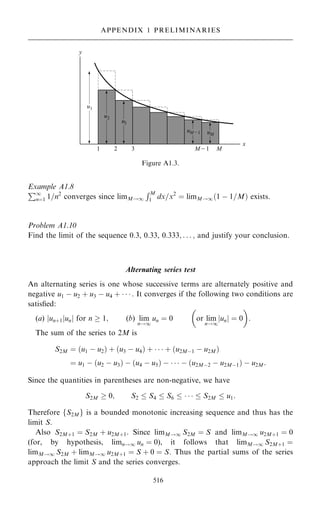
![Divide the interval [a, b] into n subintervals by means of the points
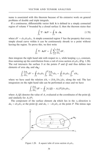
x1; x2; . . . ; xnÿ1 chosen arbitrarily. Let k be any point in the subinterval
xkÿ1 k xk, then we have
mxk f …k†xk Mxk; k ˆ 1; 2; . . . ; n;
where xk ˆ xk ÿ xkÿ1. Summing from k ˆ 1 to n and using the fact that
X
n
kˆ1
xk ˆ …x1 ÿ a† ‡ …x2 ÿ x1† ‡ ‡ …b ÿ xnÿ1† ˆ b ÿ a;
it follows that
m…b ÿ a†
X
n
rkˆ1
f …k†xk M…b ÿ a†:
Taking the limit as n ! 1 and each xk ! 0 we have the required result.
(2) If in a x b; f …x† g…x†, then
Z b
a
f …x†dx
Z b
a
g…x†dx:
(3)
Z b
a
f …x†dx
þ
þ
þ
þ
þ
þ
þ
þ
Z b
a
f …x†
j jdx if a b:
From the inequality
a ‡ b ‡ c ‡
j j a
j j ‡ b
j j ‡ c
j j ‡ ;
where jaj is the absolute value of a real number a, we have
X
n
kˆ1
f …k†xk
þ
þ
þ
þ
þ
þ
þ
þ
þ
þ
X
n
kˆ1
f …k†xk
j j ˆ
X
n
kˆ1
f …k†
j jxk:
Taking the limit as n ! 1 and each xk ! 0 we have the required result.
(4) The mean value theorem: If f …x† is continuous in [a, b], we can ®nd a point
in (a, b) such that
Z b
a
f …x†dx ˆ …b ÿ a†f …†:
Since f …x† is continuous in [a, b], we can ®nd constants m and M such that
m f …x† M. Then by (1) we have
m
1
b ÿ a
Z b
a
f …x†dx M:
Since f …x† is continuous it takes on all values between m and M; in parti-
cular there must be a value such that
f …† ˆ
Z b
a
f …x†dx=…b ÿ a†; a b:
The required result follows on multiplying by b ÿ a.
530
APPENDIX 1 PRELIMINARIES](https://image.slidesharecdn.com/mathematicalmethodsforphysicistschow-220911235848-a06d1992/85/Mathematical_Methods_for_Physicists_CHOW-pdf-545-320.jpg)