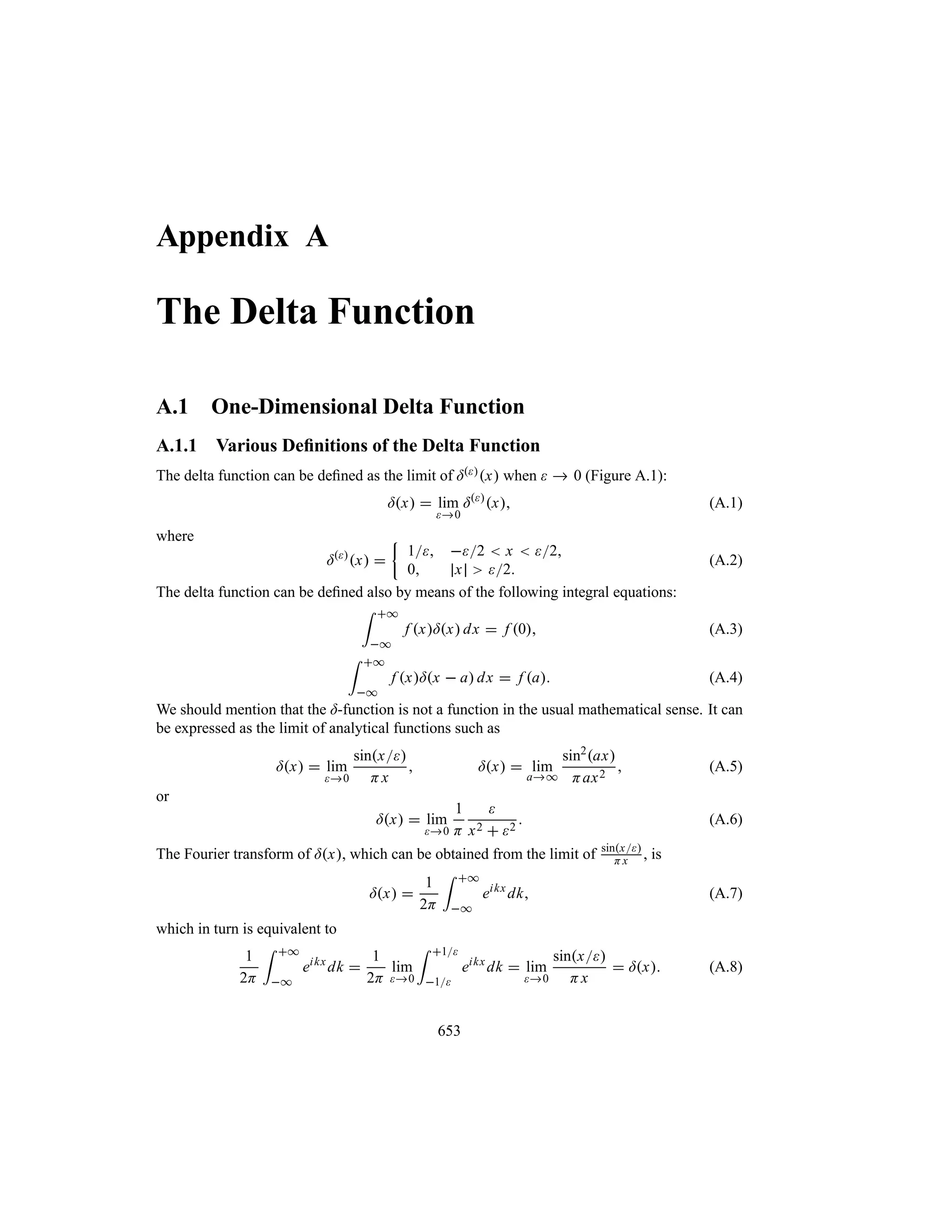
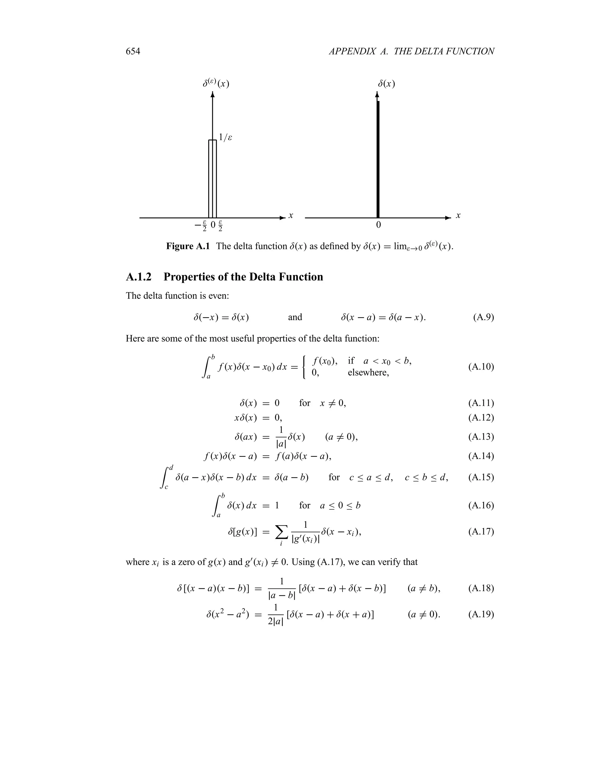
Preface to the Second Edition
It has been eight years now since the appearance of the first edition of this book in 2001. During
this time, many courteous users—professors who have been adopting the book, researchers, and
students—have taken the time and care to provide me with valuable feedback about the book.
In preparing the second edition, I have taken into consideration the generous feedback I have
received from these users. To them, and from the very outset, I want to express my deep sense
of gratitude and appreciation.
The underlying focus of the book has remained the same: to provide a well-structured and
self-contained, yet concise, text that is backed by a rich collection of fully solved examples
and problems illustrating various aspects of nonrelativistic quantum mechanics. The book is
intended to achieve a double aim: on the one hand, to provide instructors with a pedagogically
suitable teaching tool and, on the other, to help students not only master the underpinnings of
the theory but also become effective practitioners of quantum mechanics.
Although the overall structure and contents of the book have remained the same upon the
insistence of numerous users, I have carried out a number of streamlining, surgical type changes
in the second edition. These changes were aimed at fixing the weaknesses (such as typos)
detected in the first edition while reinforcing and improving on its strengths. I have introduced a
number of sections, new examples and problems, and new material; these are spread throughout
the text. Additionally, I have operated substantive revisions of the exercises at the end of the
chapters; I have added a number of new exercises, jettisoned some, and streamlined the rest.
I may underscore the fact that the collection of end-of-chapter exercises has been thoroughly
classroom tested for a number of years now.
The book has now a collection of almost six hundred examples, problems, and exercises.
Every chapter contains: (a) a number of solved examples each of which is designed to illustrate
a specific concept pertaining to a particular section within the chapter, (b) plenty of fully solved
problems (which comeat theendofeverychapter) that are generally comprehensive and, hence,
cover several concepts at once, and (c) an abundance of unsolved exercises intended for home
work assignments. Through this rich collection of examples, problems, and exercises, I want
to empower the student to become an independent learner and an adept practitioner of quantum
mechanics. Being able to solve problems is an unfailing evidence of a real understanding of the
subject.
The second edition is backed by useful resources designed for instructors adopting the book
(please contact the author or Wiley to receive these free resources).
The material in this book is suitable for three semesters—a two-semester undergraduate
course and a one-semester graduate course. A pertinent question arises: How to actually use


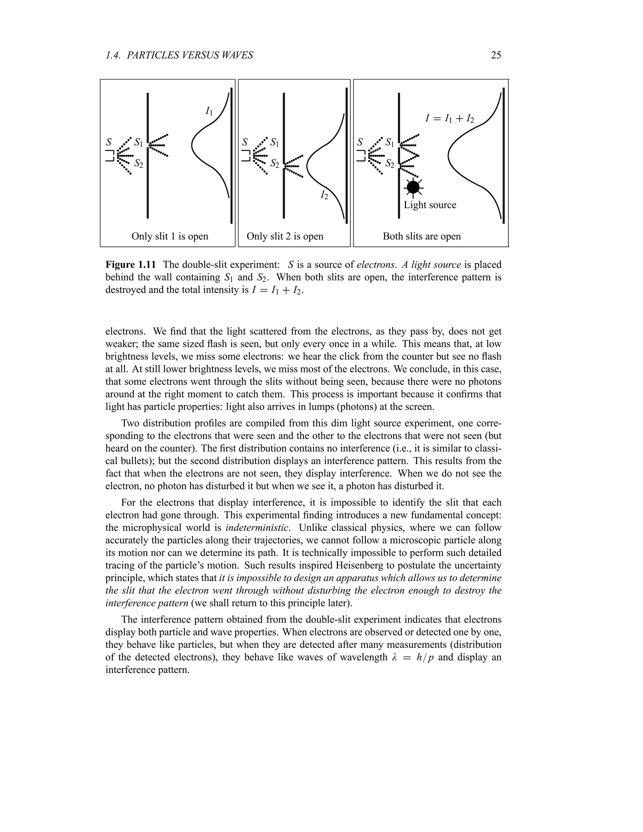

![30 CHAPTER 1. ORIGINS OF QUANTUM PHYSICS
in the measurement. So the position and momentum uncertainties are important for microscopic
systems, but negligible for macroscopic systems.
1.5.2 Probabilistic Interpretation
In quantum mechanics the state (or one of the states) of a particle is described by a wave
function O;
r t corresponding to the de Broglie wave of this particle; so O;
r t describes the
wave properties of a particle. As a result, when discussing quantum effects, it is suitable to
use the amplitude function, O, whose square modulus, O 2, is equal to the intensity of the
wave associated with this quantum effect. The intensity of a wave at a given point in space is
proportional to the probability of finding, at that point, the material particle that corresponds to
the wave.
In 1927 Born interpreted O 2 as the probability density and O;
r t 2d3r as the probability,
d P;
r t, of finding a particle at time t in the volume element d3r located between ;
r and ;
r d;
r:
O;
r t 2
d3
r d P;
r t (1.61)
where O 2 has the dimensions of [Length]3. If we integrate over the entire space, we are
certain that the particle is somewhere in it. Thus, the total probability of finding the particle
somewhere in space must be equal to one:
=
all space
O;
r t 2
d3
r 1 (1.62)
The main question now is, how does one determine the wave function O of a particle? The
answer to this question is given by the theory of quantum mechanics, where O is determined
by the Schrödinger equation (Chapters 3 and 4).
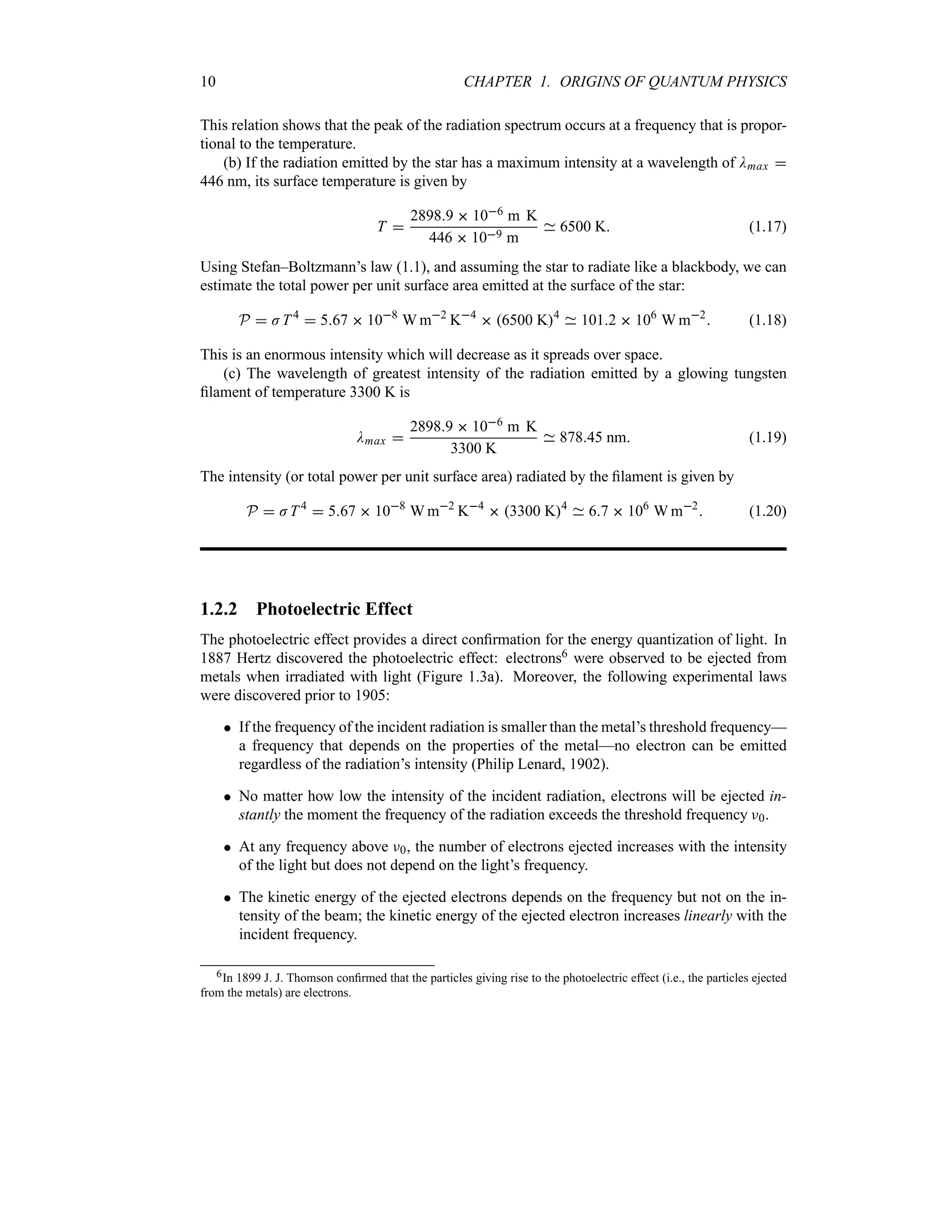
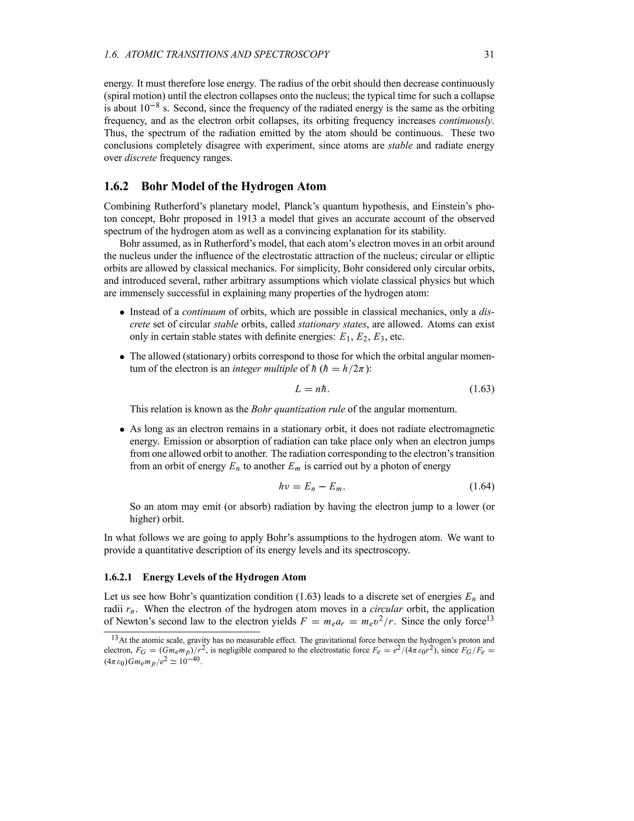
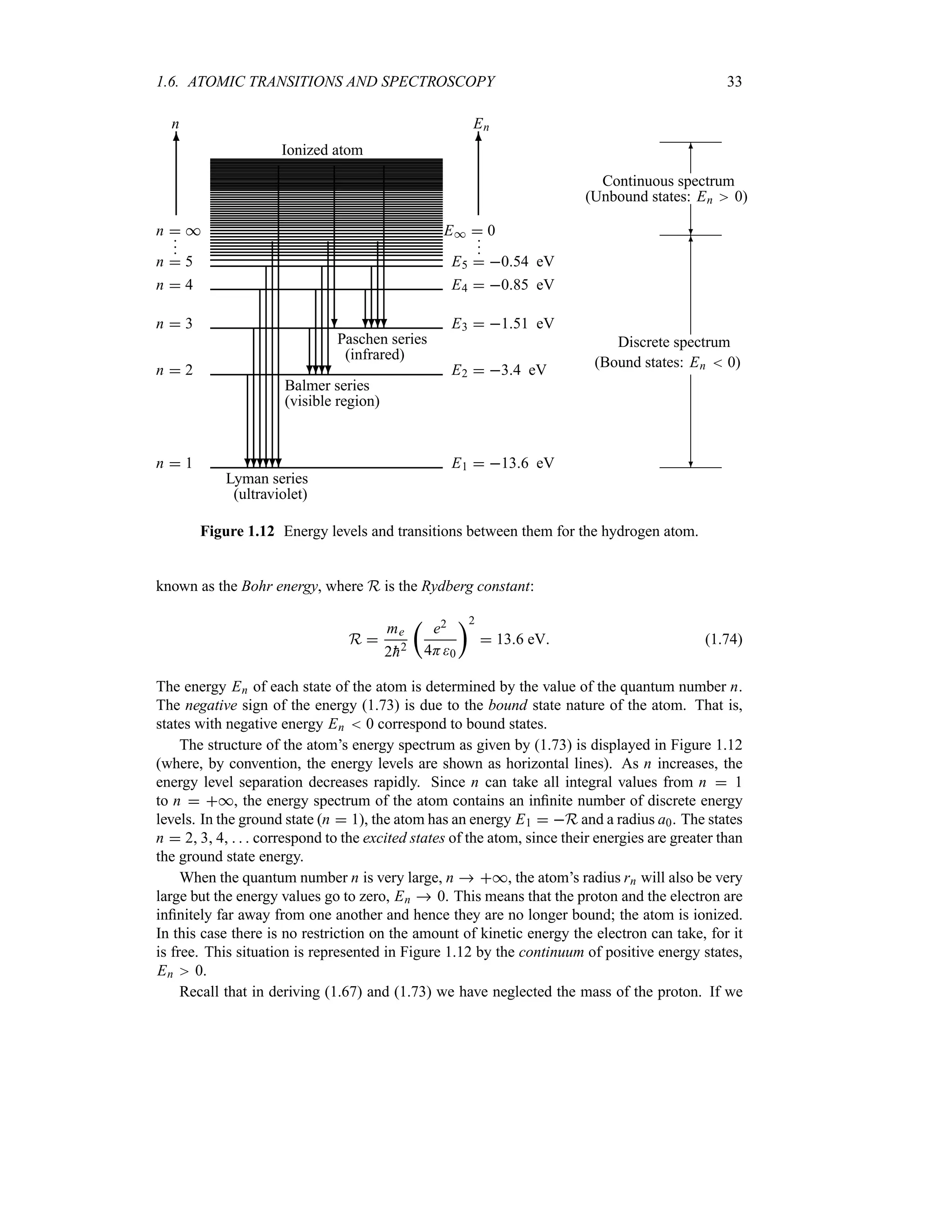
1.6 Atomic Transitions and Spectroscopy
Besides failing to explain blackbody radiation, the Compton, photoelectric, and pair production
effects and the wave–particle duality, classical physics also fails to account for many other
phenomena at the microscopic scale. In this section we consider another area where classical
physics breaks down—the atom. Experimental observations reveal that atoms exist as stable,
bound systems that have discrete numbers of energy levels. Classical physics, however, states
that any such bound system must have a continuum of energy levels.
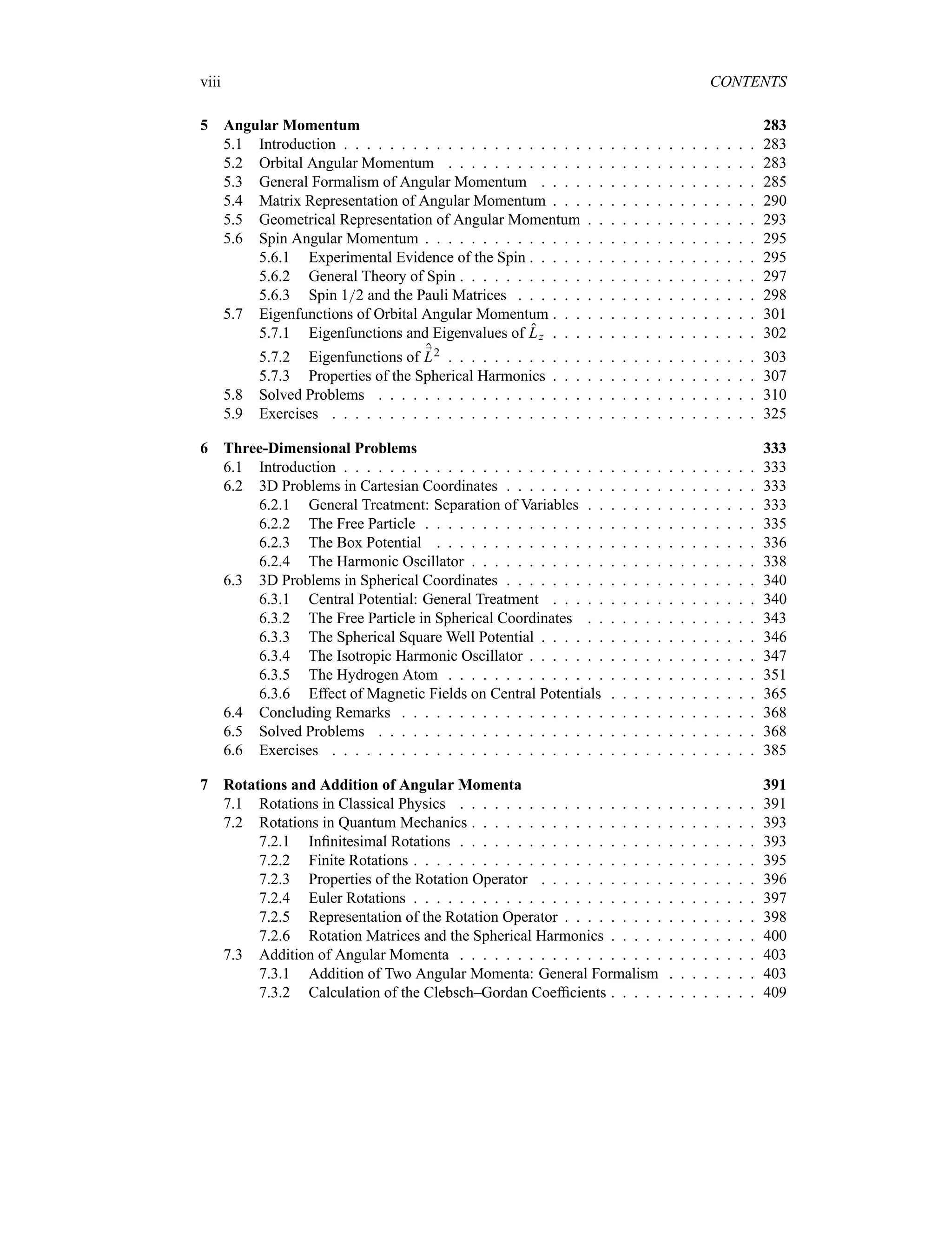
1.6.1 Rutherford Planetary Model of the Atom
After his experimental discovery of the atomic nucleus in 1911, Rutherford proposed a model
in an attempt to explain the properties of the atom. Inspired by the orbiting motion of the
planets around the sun, Rutherford considered the atom to consist of electrons orbiting around
a positively charged massive center, the nucleus. It was soon recognized that, within the context
of classical physics, this model suffers from two serious deficiencies: (a) atoms are unstable
and (b) atoms radiate energy over a continuous range of frequencies.
The first deficiency results from the application of Maxwell’s electromagnetic theory to
Rutherford’s model: as the electron orbits around the nucleus, it accelerates and hence radiates](https://image.slidesharecdn.com/zettili-250217213640-909f6141/75/Zettili-Quantum-mechanics-Concept-and-application-pdf-47-2048.jpg)

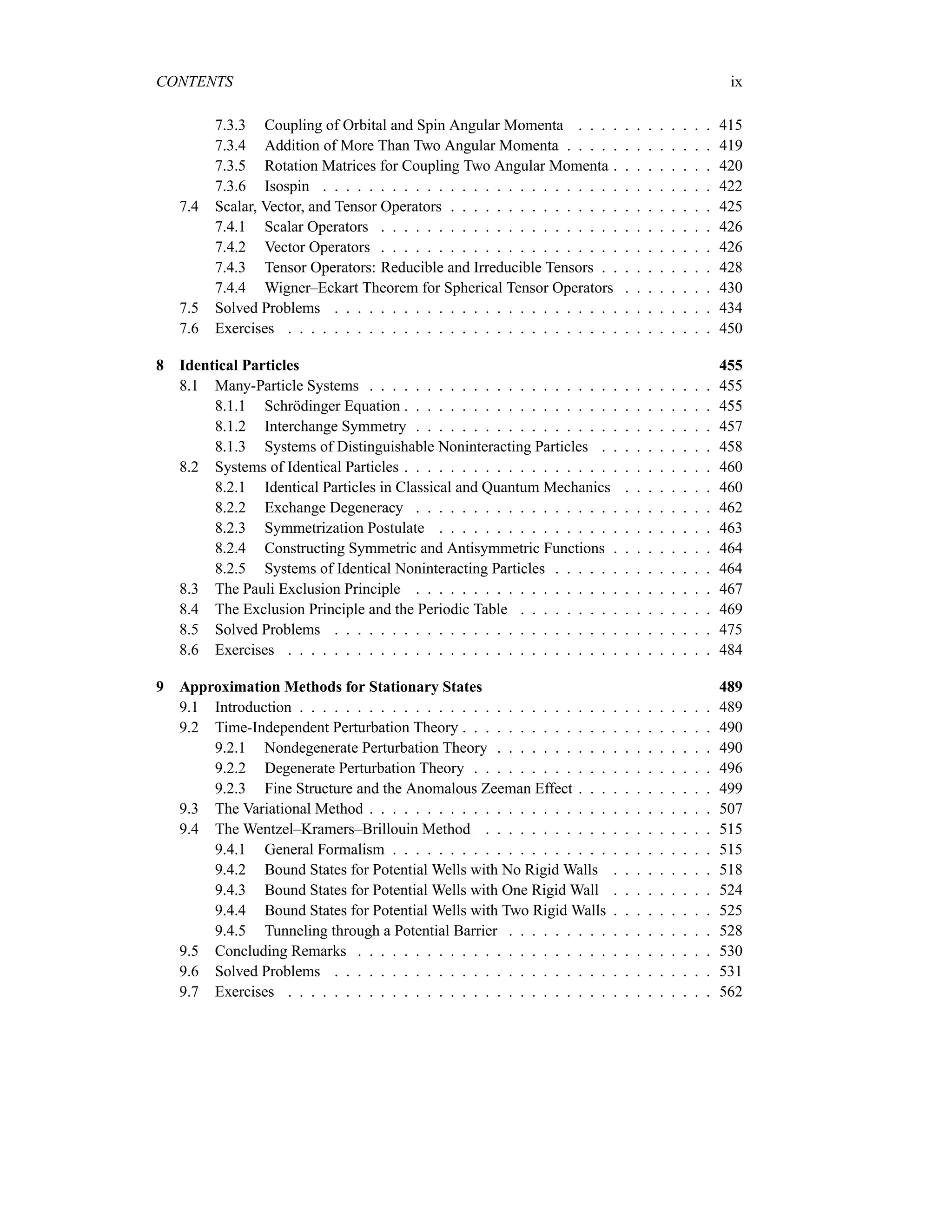
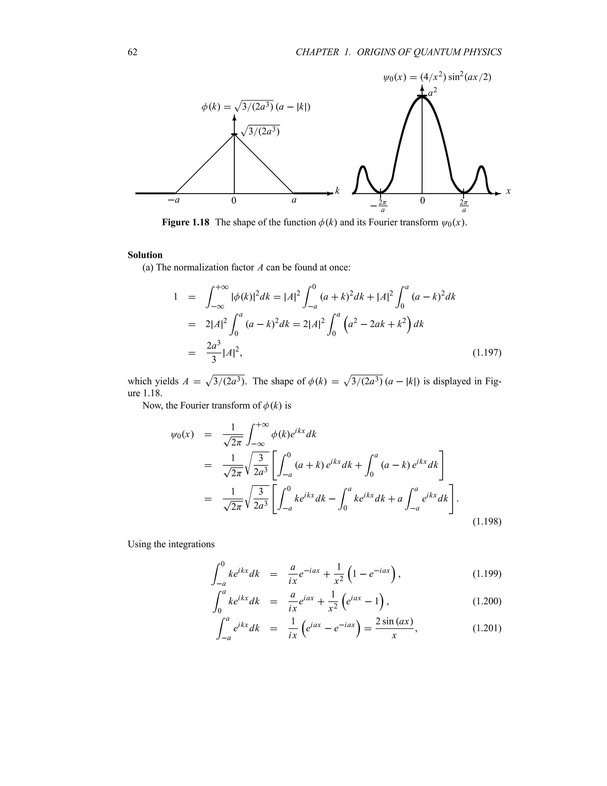
![1.8. WAVE PACKETS 41
(b) Find Mk for a square wave packet O0x
|
Aeik0x x n a
0 x a
Find the factor A so that Ox is normalized.
Solution
(a) The normalization factor A is easy to obtain:
1
= *
*
Mk 2
dk A 2
= *
*
exp
v
a2
2
k k02
w
dk (1.101)
which, by using a change of variable z k k0 and using the integral
5 *
* ea2z22dz
T
2Ha, leads at once to A
T
a
T
2H [a22H]14. Now, the wave packet corresponding
to
Mk
t
a2
2H
u14
exp
v
a2
4
k k02
w
(1.102)
is
O0x
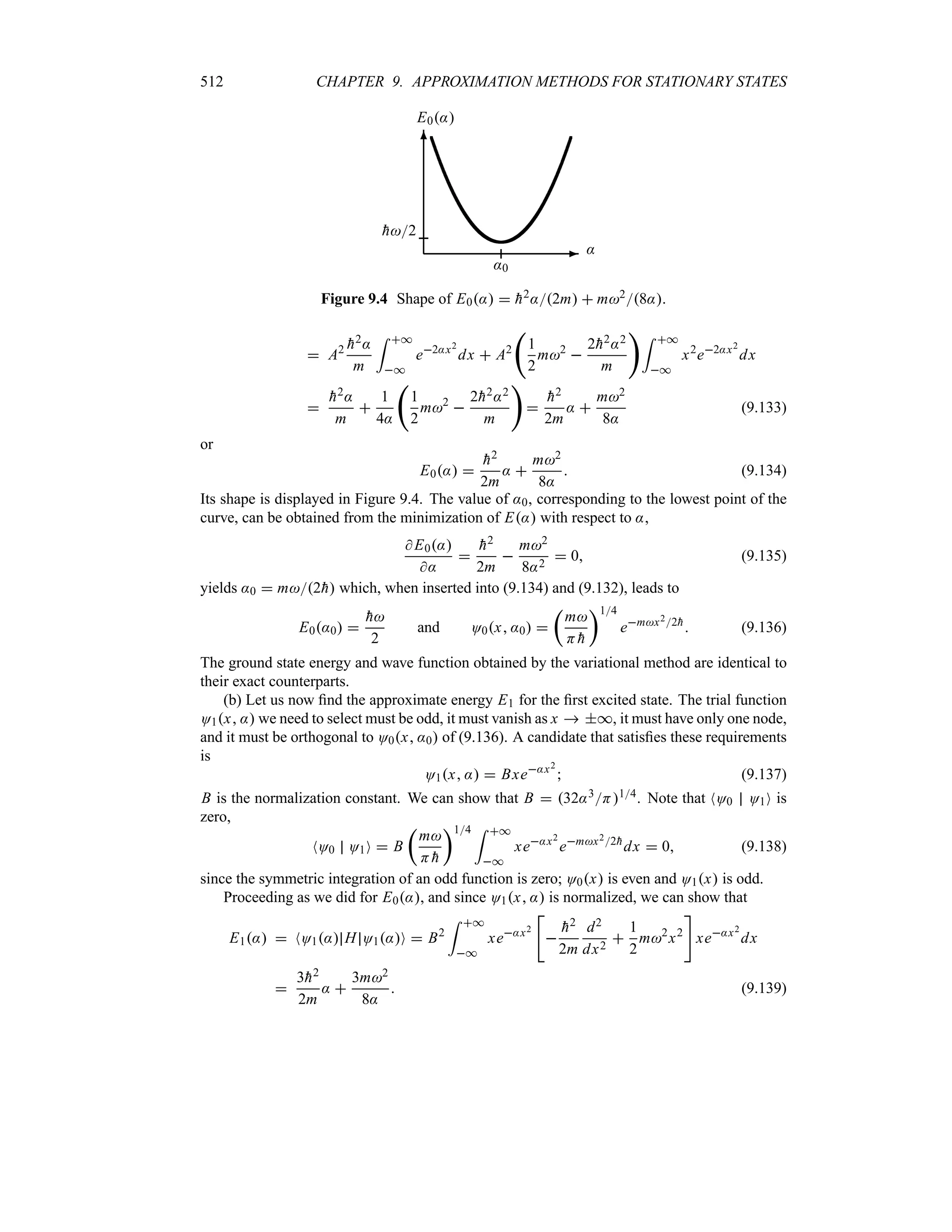
1
T
2H
= *
*
Mkeikx
dk
1
T
2H
t
a2
2H
u14 = *
*
ea2kk024ikx
dk (1.103)
To carry out the integration, we need simply to rearrange the exponent’s argument as follows:
a2
4
k k02
ikx
v
a
2
k k0
ix
a
w2
x2
a2
ik0x (1.104)
The introduction of a new variable y ak k02 ixa yields dk 2dya, and when
combined with (1.103) and (1.104), this leads to
O0x
1
T
2H
t
a2
2H
u14 = *
*
ex2a2
eik0x
ey2
t
2
a
dy
u
1
T
H
t
2
Ha2
u14
ex2a2
eik0x
= *
*
ey2
dy (1.105)
Since
5 *
* ey2
dy
T
H, this expression becomes
O0x
t
2
Ha2
u14
ex2a2
eik0x
(1.106)
where eik0x is the phase of O0x; O0x is an oscillating wave with wave number k0 modulated
by a Gaussian envelope centered at the origin. We will see later that the phase factor eik0x has
real physical significance. The wave function O0x is complex, as necessitated by quantum
mechanics. Note that O0x, like Mk, is normalized. Moreover, equations (1.102) and (1.106)
show that the Fourier transform of a Gaussian wave packet is also a Gaussian wave packet.
The probability of finding the particle in the region a2 n x n a2 can be obtained at
once from (1.106):
P
= a2
a2
O0x 2
dx
U
2
Ha2
= a2
a2
e2x2a2
dx
1
T
2H
= 1
1
ez22
dz
2
3
(1.107)](https://image.slidesharecdn.com/zettili-250217213640-909f6141/75/Zettili-Quantum-mechanics-Concept-and-application-pdf-58-2048.jpg)
![42 CHAPTER 1. ORIGINS OF QUANTUM PHYSICS
where we have used the change of variable z 2xa.
(b) The normalization of O0x is straightforward:
1
= *
*
O0x 2
dx A 2
= a
a
eik0x
eik0x
dx A 2
= a
a
dx 2a A 2
(1.108)
hence A 1
T
2a. The Fourier transform of O0x is
Mk
1
T
2H
= *
*
O0xeikx
dx
1
2
T
Ha
= a
a
eik0x
eikx
dx
1
T
Ha
sin [k k0a]
k k0
(1.109)
1.8.2 Wave Packets and the Uncertainty Relations
We want to show here that the width of a wave packet O0x and the width of its amplitude
Mk are not independent; they are correlated by a reciprocal relationship. As it turns out, the
reciprocal relationship between the widths in the x and k spaces has a direct connection to
Heisenberg’s uncertainty relation.
For simplicity, let us illustrate the main ideas on the Gaussian wave packet treated in the
previous example (see (1.102) and (1.106)):
O0x
t
2
Ha2
u14
ex2a2
eik0x
Mk
t
a2
2H
u14
ea2kk024
(1.110)
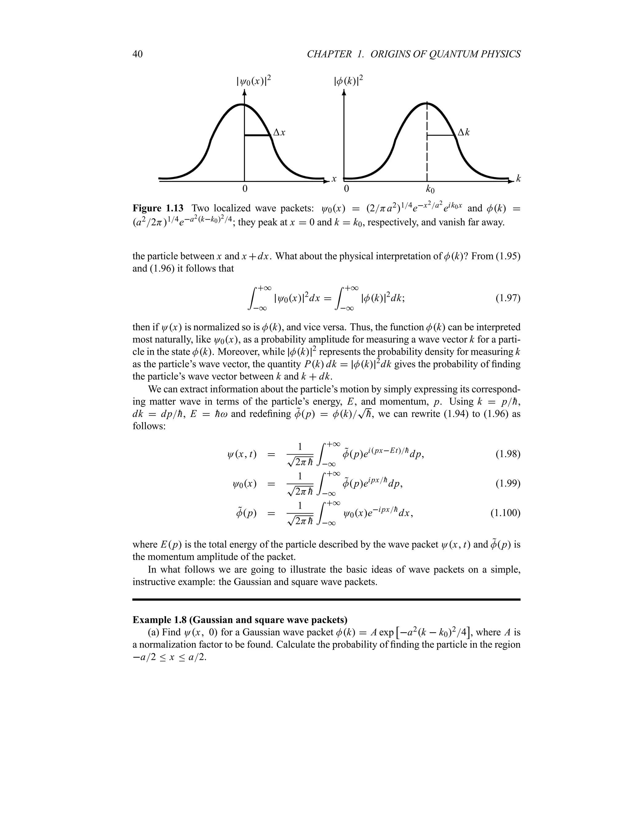
As displayed in Figure 1.13, O0x 2
and Mk 2
are centered at x 0 and k k0, respec-
tively. It is convenient to define the half-widths x and k as corresponding to the half-maxima
of O0x 2
and Mk 2
. In this way, when x varies from 0 to x and k from k0 to k0 k,
the functions O0x 2
and Mk 2
drop to e12:
Ox 0 2
O0 0 2
e12
Mk0 k 2
Mk0 2
e12
(1.111)
These equations, combined with (1.110), lead to e2x2a2
e12 and ea2k22 e12,
respectively, or to
x
a
2
k
1
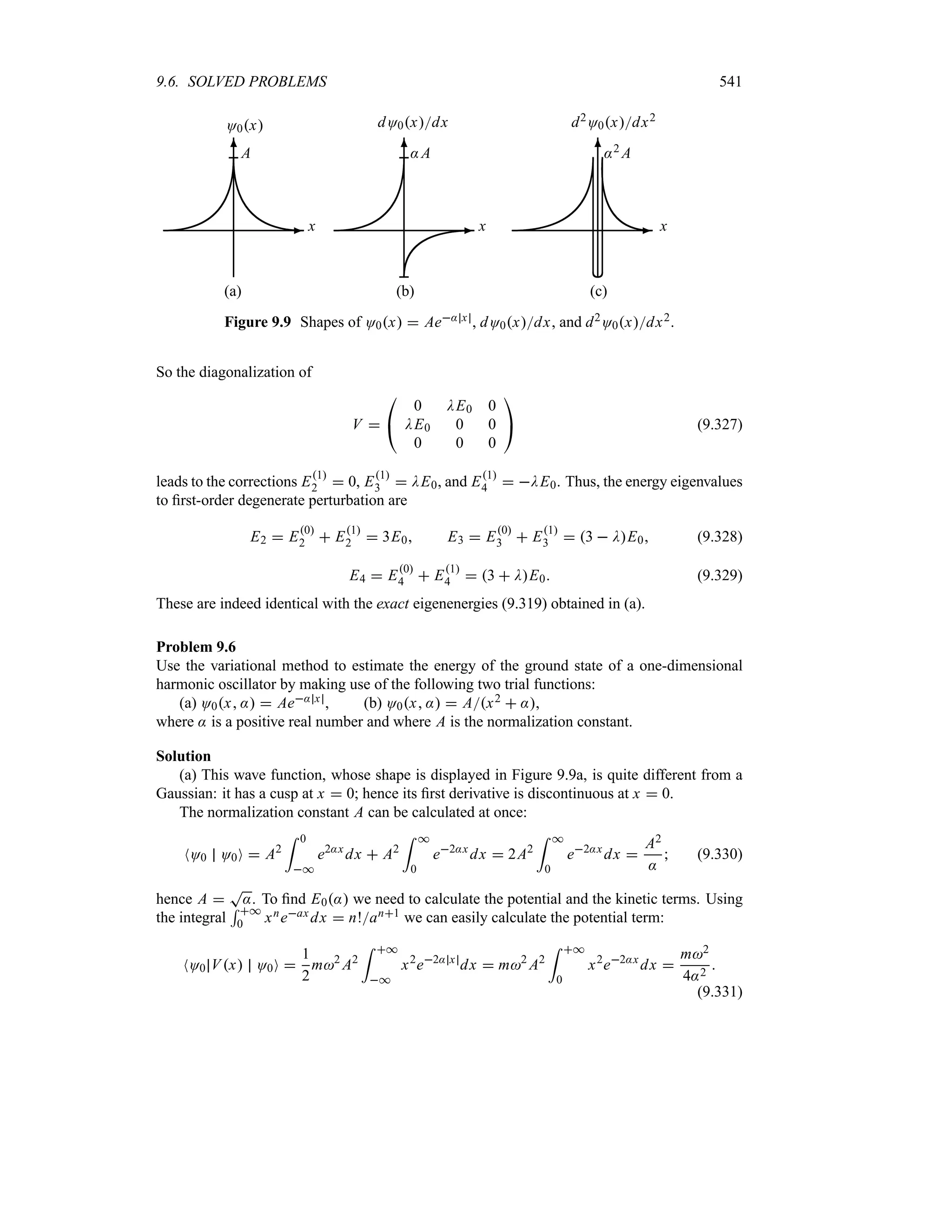
a
(1.112)
hence
xk
1
2
(1.113)
Since k p
h we have
xp
h
2
(1.114)
This relation shows that if the packet’s width is narrow in x-space, its width in momentum
space must be very broad, and vice versa.
A comparison of (1.114) with Heisenberg’s uncertainty relations (1.57) reveals that the
Gaussian wave packet yields an equality, not an inequality relation. In fact, equation (1.114) is](https://image.slidesharecdn.com/zettili-250217213640-909f6141/75/Zettili-Quantum-mechanics-Concept-and-application-pdf-59-2048.jpg)
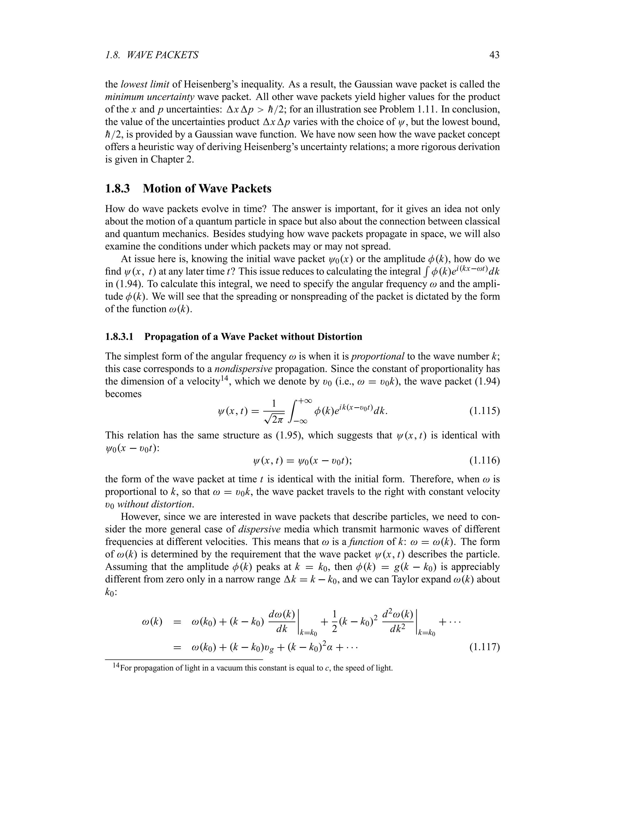


![1.8. WAVE PACKETS 47
1.8.3.2 Propagation of a Wave Packet with Distortion
Let us now include the quadratic k2 term, k k02:t, in the integrand’s exponent of (1.118)
and drop the higher terms. This leads to
Ox t eik0x)pht
f x t (1.129)
where f x t, which represents the envelope of the packet, is given by
f x t
1
T
2H
= *
*
gqeiqx)gt
eiq2:t
dq (1.130)
with q k k0. Were it not for the quadratic q2 correction, iq2:t, the wave packet would
move uniformly without any change of shape, since similarly to (1.116), f x t would be given
by f x t O0x )gt.
To show how : affects the width of the packet, let us consider the Gaussian packet (1.102)
whose amplitude is given by Mk a22H14 exp
d
a2k k024
e
and whose initial width
is x0 a2 and k
ha. Substituting Mk into (1.129), we obtain
Ox t
1
T
2H
t
a2
2H
u14
eik0x)pht
= *
*
exp
v
iqx )gt
t
a2
4
i:t
u
q2
w
dq
(1.131)
Evaluating the integral (the calculations are detailed in the following example, see Eq. (1.145)),
we can show that the packet’s density distribution is given by
Ox t 2
1
T
2Hxt
exp
b
x )gt
c2
2 [xt]2
(1.132)
where xt is the width of the packet at time t:
xt
a
2
V
1
16:2
a4
t2 x0
V
1
:2t2
x04
(1.133)
We see that the packet’s width, which was initially given by x0 a2, has grown by a factor
of
S
1 :2t2x04 after time t. Hence the wave packet is spreading; the spreading is due
to the inclusion of the quadratic q2 term, iq2:t. Should we drop this term, the packet’s width
xt would then remain constant, equal to x0.
The density distribution (1.132) displays two results: (1) the center of the packet moves
with the group velocity; (2) the packet’s width increases linearly with time. From (1.133) we
see that the packet begins to spread appreciably only when :2t2x04 s 1 or t s x02:.
In fact, if t v x02: the packet’s spread will be negligible, whereas if t w x02
: the
packet’s spread will be significant.
To be able to make concrete statements about the growth of the packet, as displayed in
(1.133), we need to specify :; this reduces to determining the function k, since :
1
2
d2
dk2
n
n
n
kk0
. For this, let us invoke an example that yields itself to explicit calculation. In
fact, the example we are going to consider—a free particle with a Gaussian amplitude—allows
the calculations to be performed exactly; hence there is no need to expand k.](https://image.slidesharecdn.com/zettili-250217213640-909f6141/75/Zettili-Quantum-mechanics-Concept-and-application-pdf-64-2048.jpg)
![1.8. WAVE PACKETS 49
Since : is a complex number (see (1.136)), we can write it in terms of its modulus and phase
:
a2
4
t
1 i
2
ht
ma2
u
a2
4
‚
1
4
h2t2
m2a4
12
eiA
(1.139)
where A tan1
d
2
htma2
e
; hence
1
T
:
2
a
‚
1
4
h2t2
m2a4
14
eiA2
(1.140)
Substituting (1.136) and (1.140) into (1.138), we have
Ox t
t
2
Ha2
u14
‚
1
4
h2t2
m2a4
14
eiA2
eik0x
hk0t2m
exp
x
hk0tm2
a2 2i
htm
(1.141)
Since
n
n
ney2a22i
htm
n
n
n
2
ey2a22i
htmey2a22i
htm, where y x
hk0tm, and
since y2a2 2i
htm y2a2 2i
htm 2a2y2a4 4
h2t2m2, we have
n
n
n
n exp
t
y2
a2 2i
htm
un
n
n
n
2
exp
t
2a2y2
a4 4
h2t2m2
u
(1.142)
hence
Ox t 2
U
2
Ha2
‚
1
4
h2t2
m2a4
12 n
n
n
n
n
exp
x
hk0tm2
a2 2i
htm
n
n
n
n
n
2
U
2
Ha2
1
t
exp
2
d
a t
e2
t
x
hk0t
m
u2
(1.143)
where t
T
1 4
h2t2m2a4.
We see that both the wave packet (1.141) and the probability density (1.143) remain Gaussian
as time evolves. This can be traced to the fact that the x-dependence of the phase, eik0x, of O0x
as displayed in (1.110) is linear. If the x-dependence of the phase were other than linear, say
quadratic, the form of the wave packet would not remain Gaussian. So the phase factor eik0x,
which was present in O0x, allows us to account for the motion of the particle.
Since the group velocity of a free particle is )g ddk d
dk
r
hk2
2m
sn
n
n
k0
hk0m, we can
rewrite (1.141) as follows17:
Ox t
1
TT
2Hxt
eiA2
eik0x)gt2
exp
b
x )gt
c2
a2 2i
htm
(1.144)
n
n
n Ox t
n
n
n
2
1
T
2Hxt
exp
b
x )gt
c2
2 [xt]2
(1.145)
17It is interesting to note that the harmonic wave eik0x)gt2 propagates with a phase velocity which is half the
group velocity; as shown in (1.124), this is a property of free particles.](https://image.slidesharecdn.com/zettili-250217213640-909f6141/75/Zettili-Quantum-mechanics-Concept-and-application-pdf-66-2048.jpg)
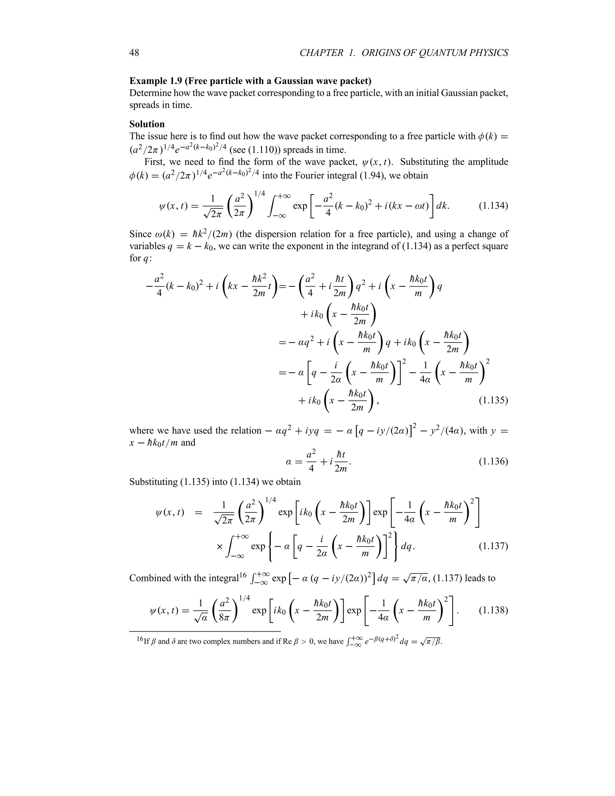
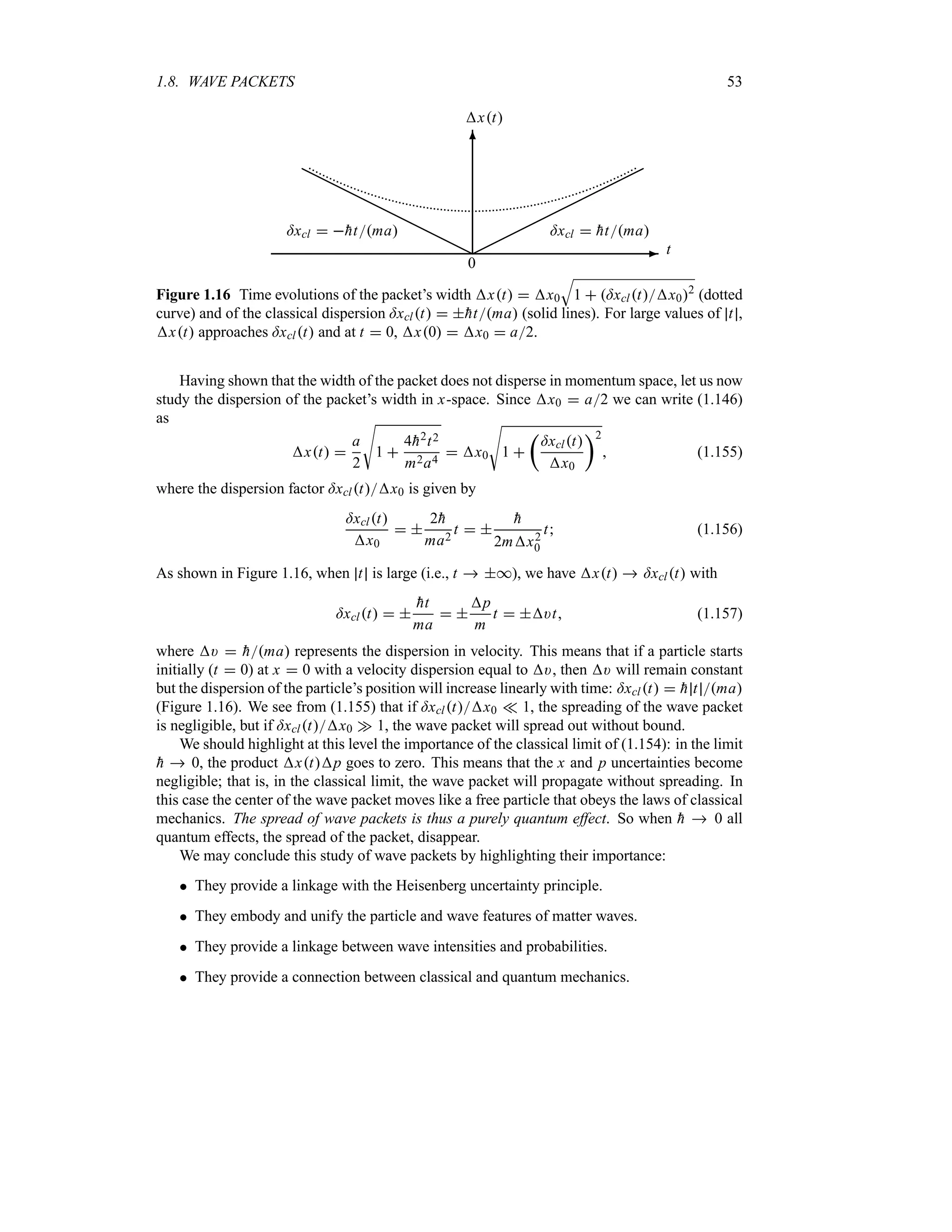
![50 CHAPTER 1. ORIGINS OF QUANTUM PHYSICS
-
6
1
T
2Hx0
T
1tK2
-
t 0
t t1
t t2
S
2Ha2
Ox t 2
)gt2 )gt1 0 )gt1 )gt2
x
- )g
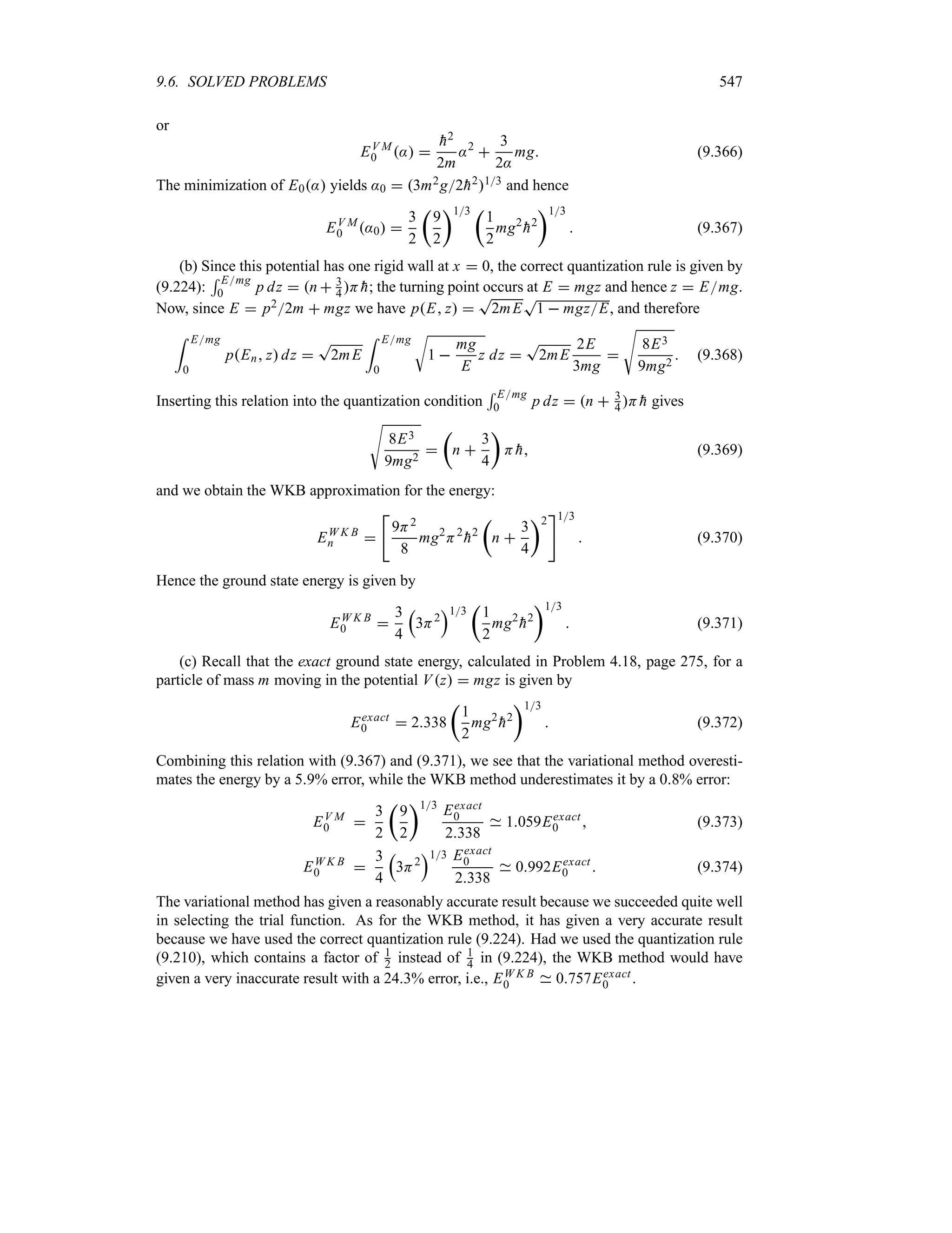
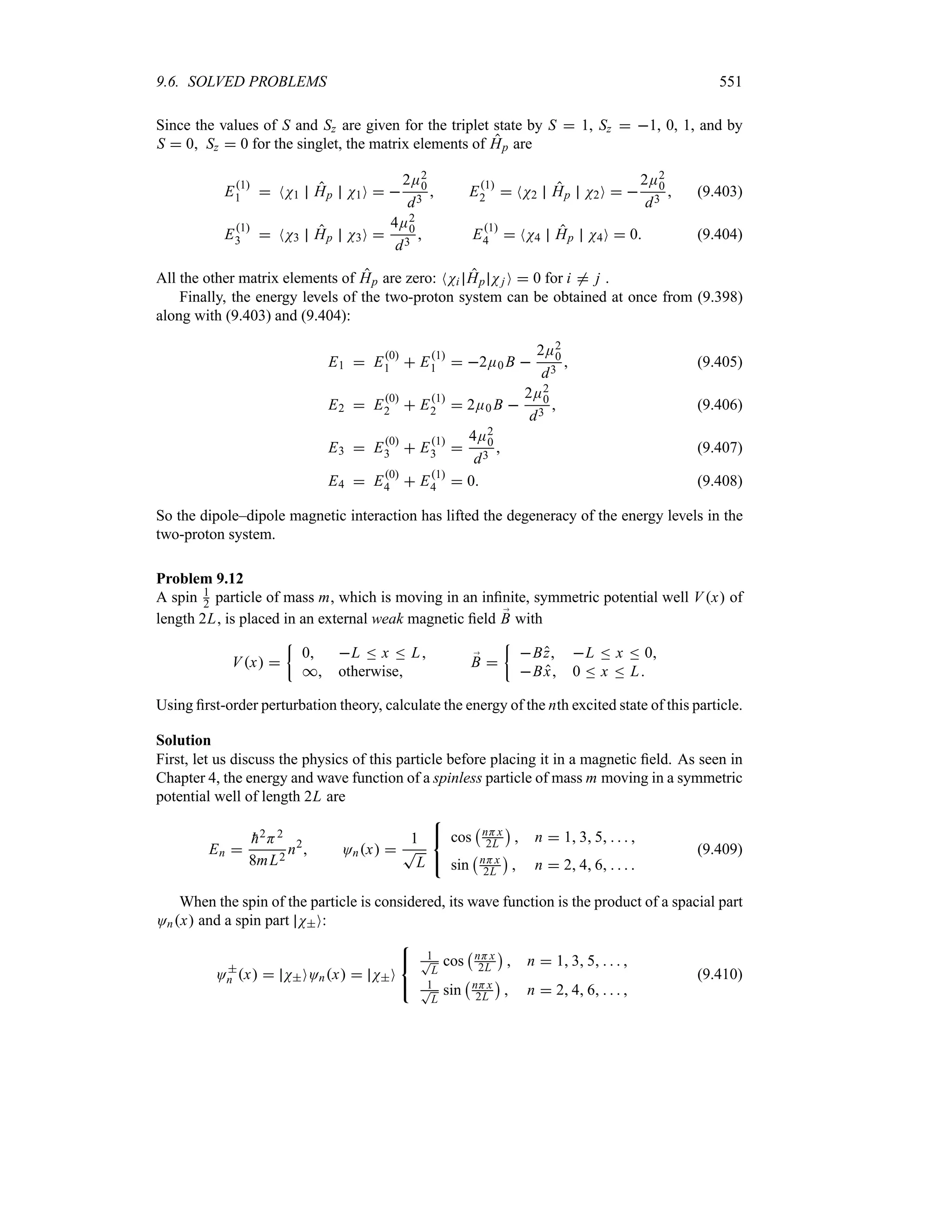
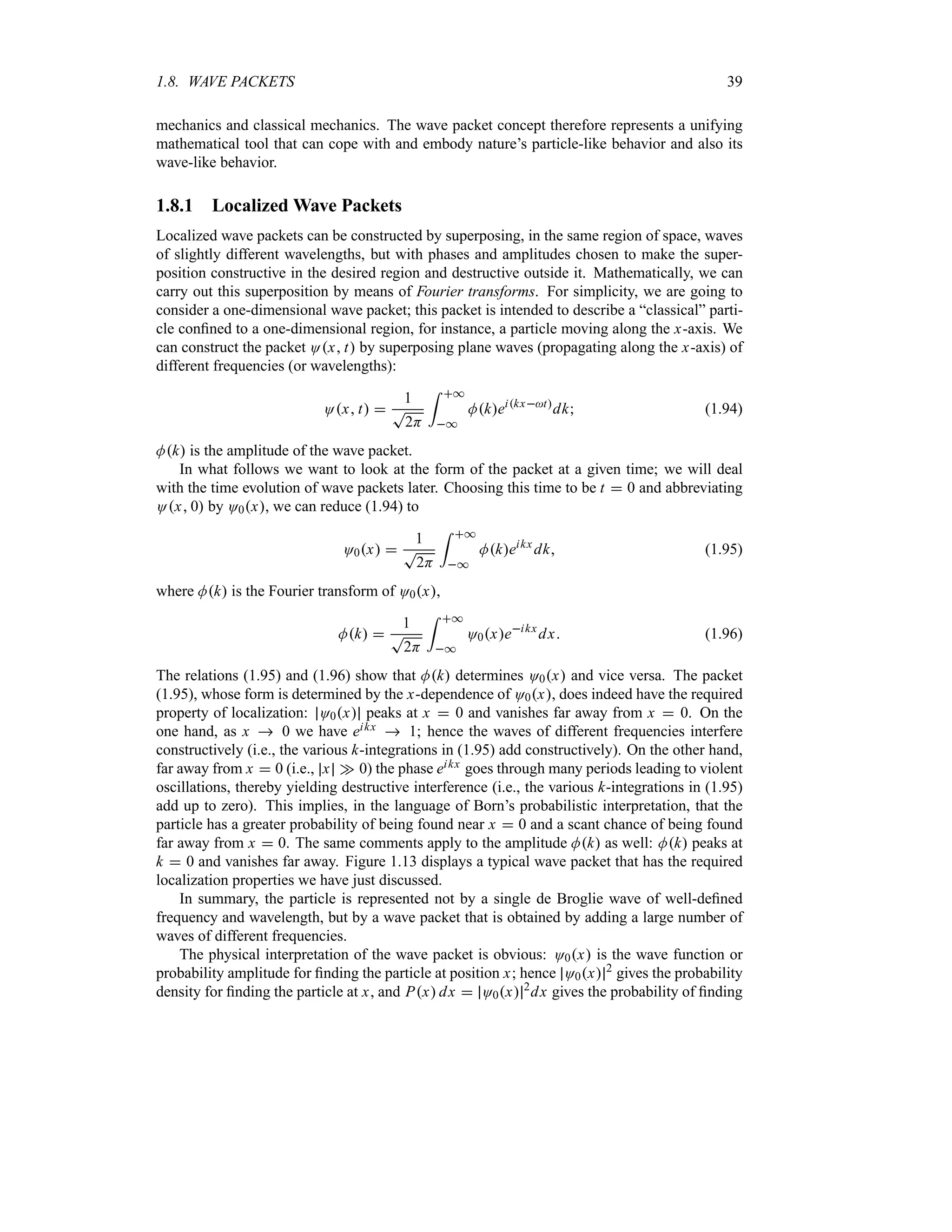
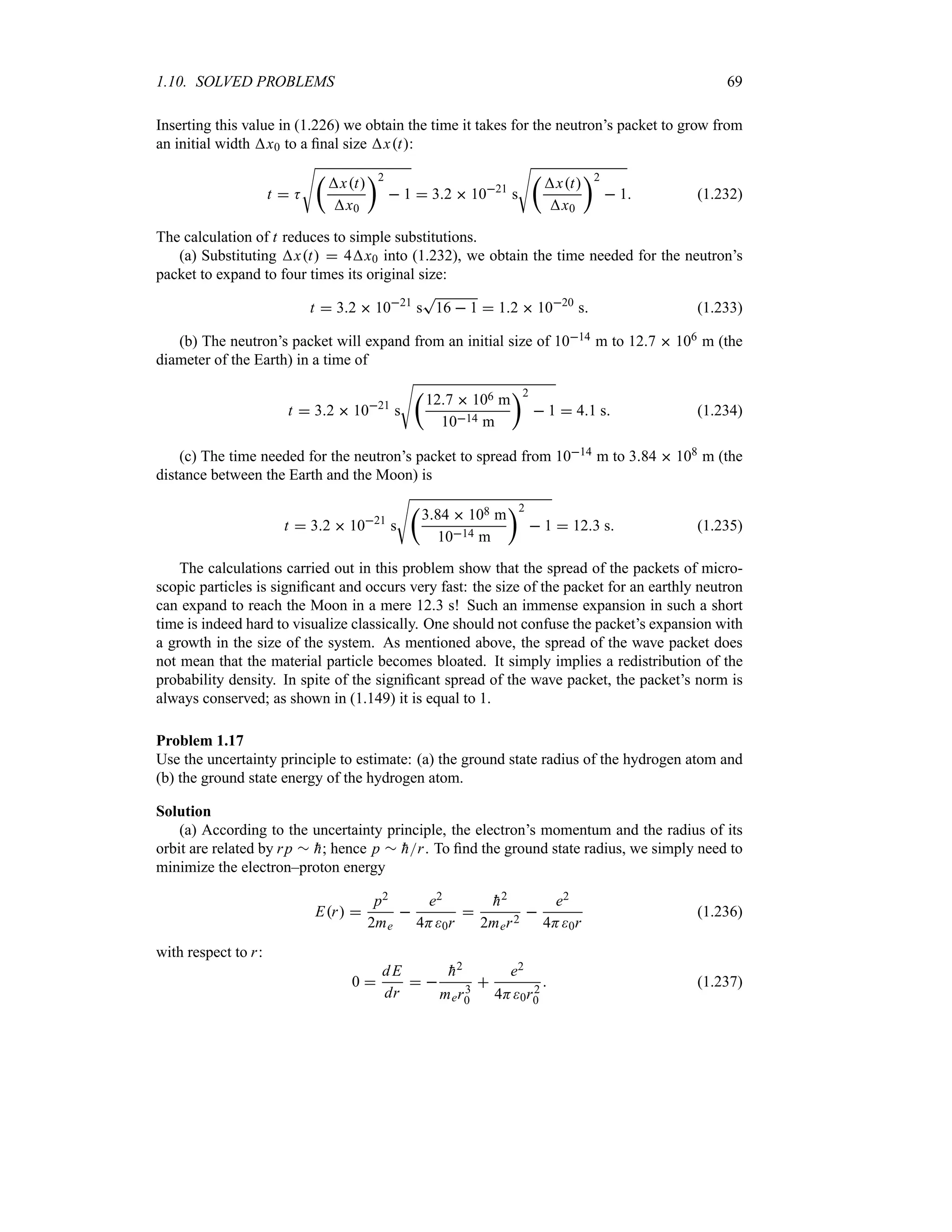
Figure 1.15 Time evolution of Ox t 2
: the peak of the packet, which is centered at x
)gt, moves with the speed )g from left to right. The height of the packet, represented here
by the dotted envelope, is modulated by the function 1
T
2Hxt, which goes to zero at
t * and is equal to
S
2Ha2 at t 0. The width of the packet xt x0
S
1 tK2
increases linearly with time.
where18
xt
a
2
t
a
2
V
1
4
h2t2
m2a4
(1.146)
represents the width of the wave packet at time t. Equations (1.144) and (1.145) describe a
Gaussian wave packet that is centered at x )gt whose peak travels with the group speed )g
hk0m and whose width xt increases linearly with time. So, during time t, the packet’s
center has moved from x 0 to x )gt and its width has expanded from x0 a2 to
xt x0
T
1 4
h2t2m2a4. The wave packet therefore undergoes a distortion; although
it remains Gaussian, its width broadens linearly with time whereas its height, 1
T
2Hxt,
decreases with time. As depicted in Figure 1.15, the wave packet, which had a very broad width
and a very small amplitude at t *, becomes narrower and narrower and its amplitude
larger and larger as time increases towards t 0; at t 0 the packet is very localized, its width
and amplitude being given by x0 a2 and
S
2Ha2, respectively. Then, as time increases
(t 0), the width of the packet becomes broader and broader, and its amplitude becomes
smaller and smaller.
In the rest of this section we are going to comment on several features that are relevant not
only to the Gaussian packet considered above but also to more general wave packets. First, let
us begin by estimating the time at which the wave packet starts to spread out appreciably. The
packet, which is initially narrow, begins to grow out noticeably only when the second term,
2
htma2, under the square root sign of (1.146) is of order unity. For convenience, let us write
18We can derive (1.146) also from (1.111): a combination of the half-width Ox t 2 O0 0 2 e12
with (1.143) yields e2[xa t]2
e12, which in turn leads to (1.146).](https://image.slidesharecdn.com/zettili-250217213640-909f6141/75/Zettili-Quantum-mechanics-Concept-and-application-pdf-67-2048.jpg)
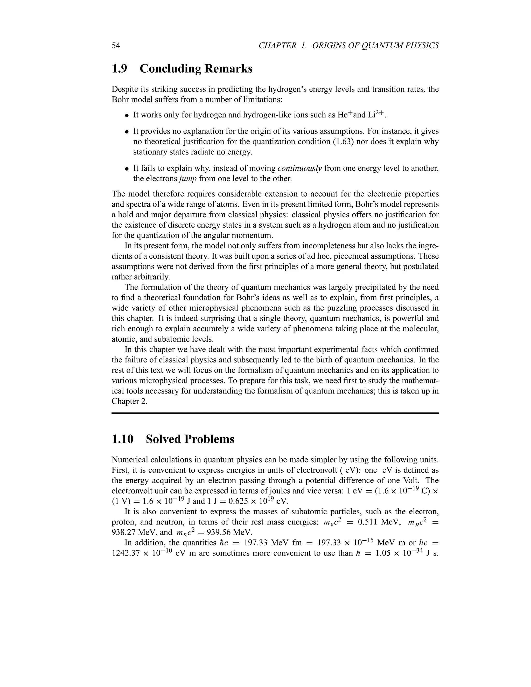
![1.10. SOLVED PROBLEMS 55
Additionally, instead of 14H0 89 109 N m2 C2, one should sometimes use the fine
structure constant : e2[4H0
hc] 1137.
Problem 1.1
A 45 kW broadcasting antenna emits radio waves at a frequency of 4 MHz.
(a) How many photons are emitted per second?
(b) Is the quantum nature of the electromagnetic radiation important in analyzing the radia-
tion emitted from this antenna?
Solution
(a) The electromagnetic energy emitted by the antenna in one second is E 45 000 J.
Thus, the number of photons emitted in one second is
n
E
hF
45 000 J
663 1034 J s 4 106 Hz
17 1031
(1.158)
(b) Since the antenna emits a huge number of photons every second, 171031, the quantum
nature of this radiation is unimportant. As a result, this radiation can be treated fairly accurately
by the classical theory of electromagnetism.
Problem 1.2
Consider a mass–spring system where a 4 kg mass is attached to a massless spring of constant
k 196 N m1; the system is set to oscillate on a frictionless, horizontal table. The mass is
pulled 25 cm away from the equilibrium position and then released.
(a) Use classical mechanics to find the total energy and frequency of oscillations of the
system.
(b) Treating the oscillator with quantum theory, find the energy spacing between two con-
secutive energy levels and the total number of quanta involved. Are the quantum effects impor-
tant in this system?
Solution
(a) According to classical mechanics, the frequency and the total energy of oscillations are
given by
F
1
2H
U
k
m
1
2H
U
196
4
111 Hz E
1
2
k A2
196
2
0252
6125 J (1.159)
(b) The energy spacing between two consecutive energy levels is given by
E hF 663 1034
J s 111 Hz 74 1034
J (1.160)
and the total number of quanta is given by
n
E
E
6125 J
74 1034 J
83 1033
(1.161)
We see that the energy of one quantum, 74 1034 J, is completely negligible compared to
the total energy 6125 J, and that the number of quanta is very large. As a result, the energy
levels of the oscillator can be viewed as continuous, for it is not feasible classically to measure
the spacings between them. Although the quantum effects are present in the system, they are
beyond human detection. So quantum effects are negligible for macroscopic systems.](https://image.slidesharecdn.com/zettili-250217213640-909f6141/75/Zettili-Quantum-mechanics-Concept-and-application-pdf-72-2048.jpg)
![58 CHAPTER 1. ORIGINS OF QUANTUM PHYSICS
(b) To obtain the angle at which the electron recoils, we need simply to use the conservation
of the total momentum along the x and y axes:
p pe cos M p)
cos A 0 pe sin M p)
sin A (1.178)
These can be rewritten as
pe cos M p p)
cos A pe sin M p)
sin A (1.179)
where p and p) are the momenta of the initial and final photons, pe is the momentum of the
recoiling electron, and A and M are the angles at which the photon and electron scatter, respec-
tively (Figure 1.4). Taking (1.179) and dividing the second equation by the first, we obtain
tan M
sin A
pp) cos A
sin A
D)D cos A
(1.180)
where we have used the momentum expressions of the incident photon p hD and of the
scattered photon p) hD). Since D 0414 nm and D) 04152 nm, the angle at which the
electron recoils is given by
M tan1
t
sin A
D)D cos A
u
tan1
t
sin 60i
041520414 cos 60i
u
5986i
(1.181)
Problem 1.6
Show that the maximum kinetic energy transferred to a proton when hit by a photon of energy
hF is Kp hF[1 mpc22hF], where mp is the mass of the proton.
Solution
Using (1.35), we have
1
F)
1
F
h
mpc2
1 cos A (1.182)
which leads to
hF)
hF
1 hFmpc21 cos A
(1.183)
Since the kinetic energy transferred to the proton is given by Kp hF hF), we obtain
Kp hF
hF
1 hFmpc21 cos A
hF
1 mpc2[hF1 cos A]
(1.184)
Clearly, the maximum kinetic energy of the proton corresponds to the case where the photon
scatters backwards (A H),
Kp
hF
1 mpc22hF
(1.185)
Problem 1.7
Consider a photon that scatters from an electron at rest. If the Compton wavelength shift is
observed to be triple the wavelength of the incident photon and if the photon scatters at 60i,
calculate
(a) the wavelength of the incident photon,
(b) the energy of the recoiling electron, and
(c) the angle at which the electron scatters.](https://image.slidesharecdn.com/zettili-250217213640-909f6141/75/Zettili-Quantum-mechanics-Concept-and-application-pdf-75-2048.jpg)
![60 CHAPTER 1. ORIGINS OF QUANTUM PHYSICS
-
6
I y
y
0
(a)
-
6
I y
y
0
(b)
Figure 1.17 Shape of the total intensity generated in a double slit experiment when both slits
are open and (a) a light source is used to observe the electrons’ motion, I y 2H1 y2,
and no interference is registered; (b) no light source is used, I y 4[H1y2] cos2Hy2,
and an interference pattern occurs.
(b) When no light source is used to observe the electrons, the motion will not be distorted
and the total intensity will be determined by an addition of the amplitudes, not the intensities:
I y O1y t O2y t 2
1
H1 y2
n
n
neikyt
eikyHyt
n
n
n
2
1
H1 y2
r
1 eiHy
s r
1 eiHy
s
4
H1 y2
cos 2
rH
2
y
s
(1.191)
The shape of this intensity does display an interference pattern which, as shown in Figure 1.17b,
results from an oscillating function, cos2Hy2, modulated by 4[H1 y2].
Problem 1.9
Consider a head-on collision between an :-particle and a lead nucleus. Neglecting the recoil
of the lead nucleus, calculate the distance of closest approach of a 90 MeV :-particle to the
nucleus.
Solution
In this head-on collision the distance of closest approach r0 can be obtained from the conserva-
tion of energy Ei E f , where Ei is the initial energy of the system, :-particle plus the lead
nucleus, when the particle and the nucleus are far from each other and thus feel no electrostatic
potential between them. Assuming the lead nucleus to be at rest, Ei is simply the energy of the
:-particle: Ei 90 MeV 9 106 16 1019 J.
As for E f , it represents the energy of the system when the :-particle is at its closest distance
from the nucleus. At this position, the :-particle is at rest and hence has no kinetic energy.
The only energy the system has is the electrostatic potential energy between the :-particle
and the lead nucleus, which has a positive charge of 82e. Neglecting the recoil of the lead](https://image.slidesharecdn.com/zettili-250217213640-909f6141/75/Zettili-Quantum-mechanics-Concept-and-application-pdf-77-2048.jpg)


![2.4. OPERATORS 89
(d) First, let us use (2.41) and (2.42) to calculate NO N O NO:
NO N O NO [1 3iNM1 5iNM2 ] [1 3i M1O 5i M2O]
1 3i1 3i 5i5i
35 (2.48)
Since NO OO 58 and NN NO 5, we infer that the triangle inequality (2.36) is satisfied:
T
35
T
58
T
5
S
NO N O NO
S
NO OO
S
NN NO (2.49)
Example 2.5
Consider two states O1O 2i M1O M2Oa M3O4 M4O and O2O 3 M1Oi M2O5 M3O M4O,
where M1O, M2O, M3O, and M4O are orthonormal kets, and where a is a constant. Find the value
of a so that O1O and O2O are orthogonal.
Solution
For the states O1O and O2O to be orthogonal, the scalar product NO2 O1O must be zero. Using
the relation NO2 3NM1 iNM2 5NM3 NM4 , we can easily find the scalar product
NO2 O1O 3NM1 iNM2 5NM3 NM4 2i M1O M2O a M3O 4 M4O
7i 5a 4 (2.50)
Since NO2 O1O 7i 5a 4 0, the value of a is a 7i 45.
2.4 Operators
2.4.1 General Definitions
Definition of an operator: An operator1 A is a mathematical rule that when applied to a ket
OO transforms it into another ket O)O of the same space and when it acts on a bra NM
transforms it into another bra NM) :
A OO O)
O NM A NM)
(2.51)
A similar definition applies to wave functions:
AO;
r O)
;
r M;
rA M)
;
r (2.52)
Examples of operators
Here are some of the operators that we will use in this text:
Unity operator: it leaves any ket unchanged, I OO OO.
The gradient operator: ;
VO;
r O;
rx;
i O;
ry;
j O;
rz;
k.
1The hat on A will be used throughout this text to distinguish an operator A from a complex number or a matrix A.](https://image.slidesharecdn.com/zettili-250217213640-909f6141/75/Zettili-Quantum-mechanics-Concept-and-application-pdf-106-2048.jpg)
![92 CHAPTER 2. MATHEMATICAL TOOLS OF QUANTUM MECHANICS
On the other hand, an operator B is said to be skew-Hermitian or anti-Hermitian if
B† B or NO B MO NM B OO`
(2.71)
Remark
The Hermitian adjoint of an operator is not, in general, equal to its complex conjugate: A
†
/
A
`
.
Example 2.6
(a) Discuss the hermiticity of the operators A A
†
, iA A
†
, and iA A
†
.
(b) Find the Hermitian adjoint of f A 1 i A 3A
2
1 2i A 9A
2
5 7A.
(c) Show that the expectation value of a Hermitian operator is real and that of an anti-
Hermitian operator is imaginary.
Solution
(a) The operator B A A
†
is Hermitian regardless of whether or not A is Hermitian,
since
B† A A
†
† A
†
A B (2.72)
Similarly, the operator iA A
†
is also Hermitian; but iA A
†
is anti-Hermitian, since
[iA A
†
]† iA A
†
.
(b) Since the Hermitian adjoint of an operator function f A is given by f †A f `A
†
,
we can write
‚
1 i A 3A
2
1 2i A 9A
2
5 7A
†
1 2i A
†
9A†
2
1 i A
†
3A†
2
5 7A
†
(2.73)
(c) From (2.70) we immediately infer that the expectation value of a Hermitian operator is
real, for it satisfies the following property:
NO A OO NO A OO`
(2.74)
that is, if A
†
A then NO A OO is real. Similarly, for an anti-Hermitian operator, B† B,
we have
NO B OO NO B OO`
(2.75)
which means that NO B OO is a purely imaginary number.
2.4.3 Projection Operators
An operator P is said to be a projection operator if it is Hermitian and equal to its own square:
P† P P2
P (2.76)
The unit operator I is a simple example of a projection operator, since I† I I2 I.](https://image.slidesharecdn.com/zettili-250217213640-909f6141/75/Zettili-Quantum-mechanics-Concept-and-application-pdf-109-2048.jpg)
![2.4. OPERATORS 93
Properties of projection operators
The product of two commuting projection operators, P1 and P2, is also a projection
operator, since
P1 P2† P
†
2 P
†
1 P2 P1 P1 P2 and P1 P22
P1 P2 P1 P2 P2
1 P2
2 P1 P2
(2.77)
The sum of two projection operators is generally not a projection operator.
Two projection operators are said to be orthogonal if their product is zero.
For a sum of projection operators P1 P2 P3 to be a projection operator, it is
necessary and sufficient that these projection operators be mutually orthogonal (i.e., the
cross-product terms must vanish).
Example 2.7
Show that the operator OONO is a projection operator only when OO is normalized.
Solution
It is easy to ascertain that the operator OONO is Hermitian, since OONO † OONO . As
for the square of this operator, it is given by
OONO 2
OONO OONO OONO OONO (2.78)
Thus, if OO is normalized, we have OONO 2
OONO . In sum, if the state OO is
normalized, the product of the ket OO with the bra NO is a projection operator.
2.4.4 Commutator Algebra
The commutator of two operators A and B, denoted by [A B], is defined by
[A B] AB B A (2.79)
and the anticommutator A B is defined by
A B AB B A (2.80)
Two operators are said to commute if their commutator is equal to zero and hence AB B A.
Any operator commutes with itself:
[A A] 0 (2.81)
Note that if two operators are Hermitian and their product is also Hermitian, these operators
commute:
AB† B†A
†
B A (2.82)
and since AB† AB we have AB B A.](https://image.slidesharecdn.com/zettili-250217213640-909f6141/75/Zettili-Quantum-mechanics-Concept-and-application-pdf-110-2048.jpg)
![94 CHAPTER 2. MATHEMATICAL TOOLS OF QUANTUM MECHANICS
As an example, we may mention the commutators involving the x-position operator, X,
and the x-component of the momentum operator, Px i
hx, as well as the y and the z
components
[X Px ] i
hI [Y Py] i
hI [Z Pz] i
hI (2.83)
where I is the unit operator.
Properties of commutators
Using the commutator relation (2.79), we can establish the following properties:
Antisymmetry:
[A B] [B A] (2.84)
Linearity:
[A B C D ] [A B] [A C] [A D] (2.85)
Hermitian conjugate of a commutator:
[A B]† [B† A
†
] (2.86)
Distributivity:
[A BC] [A B]C B[A C] (2.87)
[AB C] A[B C] [A C]B (2.88)
Jacobi identity:
[A [B C]] [B [C A]] [C [A B]] 0 (2.89)
By repeated applications of (2.87), we can show that
[A Bn
]
n1
;
j0
B j
[A B]Bn j1
(2.90)
[A
n
B]
n1
;
j0
A
n j1
[A B]A
j
(2.91)
Operators commute with scalars: an operator A commutes with any scalar b:
[A b] 0 (2.92)
Example 2.8
(a) Show that the commutator of two Hermitian operators is anti-Hermitian.
(b) Evaluate the commutator [A [B C]D].](https://image.slidesharecdn.com/zettili-250217213640-909f6141/75/Zettili-Quantum-mechanics-Concept-and-application-pdf-111-2048.jpg)
![2.4. OPERATORS 95
Solution
(a) If A and B are Hermitian, we can write
[A B]† AB B A† B†A
†
A
†
B† B A AB [A B] (2.93)
that is, the commutator of A and B is anti-Hermitian: [A B]† [A B].
(b) Using the distributivity relation (2.87), we have
[A [B C]D] [B C][A D] [A [B C]]D
BC C BAD DA ABC C BD BC C BAD
C BDA BC DA ABC D AC BD (2.94)
2.4.5 Uncertainty Relation between Two Operators
An interesting application of the commutator algebra is to derive a general relation giving the
uncertainties product of two operators, A and B. In particular, we want to give a formal deriva-
tion of Heisenberg’s uncertainty relations.
Let NAO and NBO denote the expectation values of two Hermitian operators A and B with
respect to a normalized state vector OO: NAO NO A OO and NBO NO B OO.
Introducing the operators A and B,
A A NAO B B NBO (2.95)
we have A2 A
2
2ANAO NAO2 and B2 B2 2BNBO NBO2, and hence
NO A2
OO NA2
O NA
2
O NAO2
NB2
O NB2
O NBO2
(2.96)
where NA
2
O NO A
2
OO and NB2O NO B2 OO. The uncertainties A and B are
defined by
A
T
NA2O
T
NA
2
O NAO2 B
T
NB2O
T
NB2O NBO2 (2.97)
Let us write the action of the operators (2.95) on any state OO as follows:
NO A OO
r
A NAO
s
OO MO B OO
r
B NBO
s
OO (2.98)
The Schwarz inequality for the states NO and MO is given by
NN NONM MO o NN MO 2
(2.99)
Since A and B are Hermitian, A and B must also be Hermitian: A
†
A
†
NAO
A NAO A and B† B NBO B. Thus, we can show the following three relations:
NN NO NO A2
OO NM MO NO B2
OO NN MO NO AB OO
(2.100)](https://image.slidesharecdn.com/zettili-250217213640-909f6141/75/Zettili-Quantum-mechanics-Concept-and-application-pdf-112-2048.jpg)
![96 CHAPTER 2. MATHEMATICAL TOOLS OF QUANTUM MECHANICS
For instance, since A
†
A we have NN NO NO A
†
A OO NO A2 OO
NA2O. Hence, the Schwarz inequality (2.99) becomes
NA2
ONB2
O o
n
n
nNABO
n
n
n
2
(2.101)
Notice that the last term AB of this equation can be written as
AB
1
2
[A B]
1
2
A B
1
2
[A B]
1
2
A B (2.102)
where we have used the fact that [A B] [A B]. Since [A B] is anti-Hermitian and
A B is Hermitian and since the expectation value of a Hermitian operator is real and
that the expectation value of an anti-Hermitian operator is imaginary (see Example 2.6), the
expectation value NABO of (2.102) becomes equal to the sum of a real part N A B O2
and an imaginary part N[A B]O2; hence
n
n
nNABO
n
n
n
2
1
4
n
n
nN[A B]O
n
n
n
2
1
4
n
n
nN A B O
n
n
n
2
(2.103)
Since the last term is a positive real number, we can infer the following relation:
n
n
nNABO
n
n
n
2
o
1
4
n
n
nN[A B]O
n
n
n
2
(2.104)
Comparing equations (2.101) and (2.104), we conclude that
NA2
ONB2
O o
1
4
n
n
nN[A B]O
n
n
n
2
(2.105)
which (by taking its square root) can be reduced to
AB o
1
2
n
n
nN[A B]O
n
n
n (2.106)
This uncertainty relation plays an important role in the formalism of quantum mechanics. Its
application to position and momentum operators leads to the Heisenberg uncertainty relations,
which represent one of the cornerstones of quantum mechanics; see the next example.
Example 2.9 (Heisenberg uncertainty relations)
Find the uncertainty relations between the components of the position and the momentum op-
erators.
Solution
By applying (2.106) to the x-components of the position operator X, and the momentum op-
erator Px , we obtain xpx o 1
2 N[X Px ]O . But since [X Px ] i
hI, we have
xpx o
h2; the uncertainty relations for the y and z components follow immediately:
xpx o
h
2
ypy o
h
2
zpz o
h
2
(2.107)
These are the Heisenberg uncertainty relations.](https://image.slidesharecdn.com/zettili-250217213640-909f6141/75/Zettili-Quantum-mechanics-Concept-and-application-pdf-113-2048.jpg)
![2.4. OPERATORS 97
2.4.6 Functions of Operators
Let FA be a function of an operator A. If A is a linear operator, we can Taylor expand FA
in a power series of A:
FA
*
;
n0
an A
n
(2.108)
where an is just an expansion coefficient. As an illustration of an operator function, consider
eaA, where a is a scalar which can be complex or real. We can expand it as follows:
eaA
*
;
n0
an
n!
A
n
I aA
a2
2!
A
2
a3
3!
A
3
(2.109)
Commutators involving function operators
If A commutes with another operator B, then B commutes with any operator function that
depends on A:
[A B] 0 [B FA] 0 (2.110)
in particular, FA commutes with A and with any other function, GA, of A:
[A FA] 0 [A
n
FA] 0 [FA GA] 0 (2.111)
Hermitian adjoint of function operators
The adjoint of FA is given by
[FA]† F`
A
†
(2.112)
Note that if A is Hermitian, FA is not necessarily Hermitian; FA will be Hermitian only if
F is a real function and A is Hermitian. An example is
eA
† eA
†
ei A
† ei A†
ei:A
† ei:` A†
(2.113)
where : is a complex number. So if A is Hermitian, an operator function which can be ex-
panded as FA
3*
n0 an A
n
will be Hermitian only if the expansion coefficients an are real
numbers. But in general, FA is not Hermitian even if A is Hermitian, since
F`
A
†
*
;
n0
a`
nA†n
(2.114)
Relations involving function operators
Note that
[A B] / 0 [B FA] / 0 (2.115)
in particular, eAeB / eAB. Using (2.109) we can ascertain that
eA
eB
eAB
e[A B]2
(2.116)
eA
BeA
B [A B]
1
2!
[A [A B]]
1
3!
[A [A [A B]]] (2.117)](https://image.slidesharecdn.com/zettili-250217213640-909f6141/75/Zettili-Quantum-mechanics-Concept-and-application-pdf-114-2048.jpg)
![2.4. OPERATORS 99
Solution
Clearly, if is real and G is Hermitian, the operator eiG would be unitary. Using the property
[FA]† F`A
†
, we see that
eiG
† eiG
eiG
1
(2.125)
that is, U† U1.
2.4.8 Eigenvalues and Eigenvectors of an Operator
Having studied the properties of operators and states, we are now ready to discuss how to find
the eigenvalues and eigenvectors of an operator.
A state vector OO is said to be an eigenvector (also called an eigenket or eigenstate) of an
operator A if the application of A to OO gives
A OO a OO (2.126)
where a is a complex number, called an eigenvalue of A. This equation is known as the eigen-
value equation, or eigenvalue problem, of the operator A. Its solutions yield the eigenvalues
and eigenvectors of A. In Section 2.5.3 we will see how to solve the eigenvalue problem in a
discrete basis.
A simple example is the eigenvalue problem for the unity operator I:
I OO OO (2.127)
This means that all vectors are eigenvectors of I with one eigenvalue, 1. Note that
A OO a OO An
OO an
OO and FA OO Fa OO (2.128)
For instance, we have
A OO a OO ei A
OO eia
OO (2.129)
Example 2.11 (Eigenvalues of the inverse of an operator)
Show that if A
1
exists, the eigenvalues of A
1
are just the inverses of those of A.
Solution
Since A
1
A I we have on the one hand
A
1
A OO OO (2.130)
and on the other hand
A
1
A OO A
1
A OO aA
1
OO (2.131)
Combining the previous two equations, we obtain
aA
1
OO OO (2.132)](https://image.slidesharecdn.com/zettili-250217213640-909f6141/75/Zettili-Quantum-mechanics-Concept-and-application-pdf-116-2048.jpg)
![102 CHAPTER 2. MATHEMATICAL TOOLS OF QUANTUM MECHANICS
2.4.9.1 Unitary Transformations
Kets OO and bras NO transform as follows:
O)
O U OO NO)
NO U† (2.144)
Let us now find out how operators transform under unitary transformations. Since the transform
of A OO MO is A
)
O)O M)O, we can rewrite A
)
O)O M)O as A
)
U OO U MO
U A OO which, in turn, leads to A
)
U U A. Multiplying both sides of A
)
U U A by U† and
since UU† U†U I, we have
A
)
U AU† A U†A
)
U (2.145)
The results reached in (2.144) and (2.145) may be summarized as follows:
O)
O U OO NO)
NO U† A
)
U AU† (2.146)
OO U† O)
O NO NO)
U A U†A
)
U (2.147)
Properties of unitary transformations
If an operator A is Hermitian, its transformed A
)
is also Hermitian, since
A
) † U AU†† U A
†
U† U AU† A
)
(2.148)
The eigenvalues of A and those of its transformed A
)
are the same:
A OnO an OnO A
)
O)
nO an O)
nO (2.149)
since
A
)
O)
nO U AU†U OnO U AU†U OnO
U A OnO anU OnO an O)
nO (2.150)
Commutators that are equal to (complex) numbers remain unchanged under unitary trans-
formations, since the transformation of [A B] a, where a is a complex number, is
given by
[A
)
B)
] [U AU†U BU†] U AU†U BU† U BU†U AU†
U[A B]U† UaU† aUU† a
[A B] (2.151)
We can also verify the following general relations:
A ;B C A
)
;B)
C)
(2.152)
A :BC D A
)
:B)
C)
D)
(2.153)
where A
)
, B), C), and D) are the transforms of A, B, C, and D, respectively.](https://image.slidesharecdn.com/zettili-250217213640-909f6141/75/Zettili-Quantum-mechanics-Concept-and-application-pdf-119-2048.jpg)
![104 CHAPTER 2. MATHEMATICAL TOOLS OF QUANTUM MECHANICS
where
= OO iG OO (2.163)
The transformation of an operator A is given by
A
)
I iGAI iG A i[G A] (2.164)
If G commutes with A, the unitary transformation will leave A unchanged, A
)
A:
[G A] 0 A
)
I iGAI iG A (2.165)
2.4.9.3 Finite Unitary Transformations
We can construct a finite unitary transformation from (2.160) by performing a succession of
infinitesimal transformations in steps of ; the application of a series of successive unitary
transformations is equivalent to the application of a single unitary transformation. Denoting
:N, where N is an integer and : is a finite parameter, we can apply the same unitary
transformation N times; in the limit N * we obtain
U:G lim
N*
N
k1
r
1 i
:
N
G
s
lim
N*
r
1 i
:
N
G
sN
ei:G
(2.166)
where G is now the generator of the finite transformation and : is its parameter.
As shown in (2.125), U is unitary only when the parameter : is real and G is Hermitian,
since
ei:G
† ei:G
ei:G
1
(2.167)
Using the commutation relation (2.117), we can write the transformation A
)
of an operator A
as follows:
ei:G
Aei:G
A i:[G A]
i:2
2!
K
G [G A]
L
i:3
3!
K
G [G [G A]]
L
(2.168)
If G commutes with A, the unitary transformation will leave A unchanged, A
)
A:
[G A] 0 A
)
ei:G
Aei:G
A (2.169)
In Chapter 3, we will consider some important applications of infinitesimal unitary transfor-
mations to study time translations, space translations, space rotations, and conservation laws.
2.5 Representation in Discrete Bases
By analogy with the expansion of Euclidean space vectors in terms of the basis vectors, we need
to express any ket OO of the Hilbert space in terms of a complete set of mutually orthonormal
base kets. State vectors are then represented by their components in this basis.](https://image.slidesharecdn.com/zettili-250217213640-909f6141/75/Zettili-Quantum-mechanics-Concept-and-application-pdf-121-2048.jpg)
![2.5. REPRESENTATION IN DISCRETE BASES 111
Example 2.14
(a) Show that TrAB TrB A.
(b) Show that the trace of a commutator is always zero.
(c) Illustrate the results shown in (a) and (b) on the following matrices:
A
#
8 2i 4i 0
1 0 1 i
8 i 6i
$ B
#
i 2 1 i
6 1 i 3i
1 5 7i 0
$
Solution
(a) Using the definition of the trace,
TrAB
;
n
NMn AB MnO (2.207)
and inserting the unit operator between A and B we have
TrAB
;
n
NMn A
‚
;
m
MmONMm
B MnO
;
nm
NMn A MmONMm B MnO
;
nm
Anm Bmn (2.208)
On the other hand, since TrAB
3
nNMn AB MnO, we have
TrB A
;
m
NMm B
‚
;
n
MnONMn
A MmO
;
m
NMm B MnONMn A MmO
;
nm
Bmn Anm (2.209)
Comparing (2.208) and (2.209), we see that TrAB TrB A.
(b) Since TrAB TrB A we can infer at once that the trace of any commutator is always
zero:
Tr[A B] TrAB TrB A 0 (2.210)
(c) Let us verify that the traces of the products AB and B A are equal. Since
AB
#
2 16i 12 6 10i
1 2i 14 2i 1 i
20i 59 31i 11 8i
$ B A
#
8 5 i 8 4i
49 35i 3 24i 16
13 5i 4i 12 2i
$
(2.211)
we have
TrAB Tr
#
2 16i 12 6 10i
1 2i 14 2i 1 i
20i 59 31i 11 8i
$ 1 26i (2.212)
TrB A Tr
#
8 5 i 8 4i
49 35i 3 24i 16
13 5i 4i 12 2i
$ 1 26i TrAB (2.213)
This leads to TrAB TrB A 1 26i 1 26i 0 or Tr[A B] 0.](https://image.slidesharecdn.com/zettili-250217213640-909f6141/75/Zettili-Quantum-mechanics-Concept-and-application-pdf-128-2048.jpg)


![118 CHAPTER 2. MATHEMATICAL TOOLS OF QUANTUM MECHANICS
where a is a complex number. Inserting the unit operator between A and OO and multiplying
by NMm , we can cast the eigenvalue equation in the form
NMm A
‚
;
n
MnONMn
OO aNMm
‚
;
n
MnONMn
OO (2.253)
or ;
n
AmnNMn OO a
;
n
NMn OO=nm (2.254)
which can be rewritten as ;
n
[Amn a=nm] NMn OO 0 (2.255)
with Amn NMm A MnO.
This equation represents an infinite, homogeneous system of equations for the coefficients
NMn OO, since the basis MnO is made of an infinite number of base kets. This system of
equations can have nonzero solutions only if its determinant vanishes:
det Amn a=nm 0 (2.256)
The problem that arises here is that this determinant corresponds to a matrix with an infinite
number of columns and rows. To solve (2.256) we need to truncate the basis MnO and assume
that it contains only N terms, where N must be large enough to guarantee convergence. In this
case we can reduce (2.256) to the following Nth degree determinant:
n
n
n
n
n
n
n
n
n
n
n
A11 a A12 A13 A1N
A21 A22 a A23 A2N
A31 A32 A33 a A3N
AN1 AN2 AN3 AN N a
n
n
n
n
n
n
n
n
n
n
n
0 (2.257)
This is known as the secular or characteristic equation. The solutions of this equation yield
the N eigenvalues a1, a2, a3, , aN , since it is an Nth order equation in a. The set of these
N eigenvalues is called the spectrum of A. Knowing the set of eigenvalues a1, a2, a3, , aN ,
we can easily determine the corresponding set of eigenvectors M1O, M2O, , MN O. For
each eigenvalue am of A, we can obtain from the “secular” equation (2.257) the N components
NM1 OO, NM2 OO, NM3 OO, , NMN OO of the corresponding eigenvector MmO.
If a number of different eigenvectors (two or more) have the same eigenvalue, this eigen-
value is said to be degenerate. The order of degeneracy is determined by the number of linearly
independent eigenvectors that have the same eigenvalue. For instance, if an eigenvalue has five
different eigenvectors, it is said to be fivefold degenerate.
In the case where the set of eigenvectors MnO of A is complete and orthonormal, this set
can be used as a basis. In this basis the matrix representing the operator A is diagonal,
A
%
%
%
#
a1 0 0
0 a2 0
0 0 a3
$
(2.258)](https://image.slidesharecdn.com/zettili-250217213640-909f6141/75/Zettili-Quantum-mechanics-Concept-and-application-pdf-135-2048.jpg)

![2.6. REPRESENTATION IN CONTINUOUS BASES 127
2.6.4.3 Important Commutation Relations
Let us now calculate the commutator [Rj Pk] in the position representation. As the separate
actions of X Px and Px X on the wave function O;
r are given by
X Px O;
r i
hx
O;
r
x
(2.318)
Px XO;
r i
h
x
xO;
r i
hO;
r i
hx
O;
r
x
(2.319)
we have
[X Px]O;
r X Px O;
r Px XO;
r i
hx
O;
r
x
i
hO;
r i
hx
O;
r
x
i
hO;
r (2.320)
or
[X Px] i
h (2.321)
Similar relations can be derived at once for the y and the z components:
[X Px ] i
h [Y PY ] i
h [Z PZ ] i
h (2.322)
We can verify that
[X Py] [X Pz] [Y Px] [Y Pz] [Z Px] [Z Py] 0 (2.323)
since the x, y, z degrees of freedom are independent; the previous two relations can be grouped
into
[Rj Pk] i
h=jk [Rj Rk] 0 [Pj Pk] 0 j k x y z (2.324)
These relations are often called the canonical commutation relations.
Now, from (2.321) we can show that (for the proof see Problem 2.8 on page 139)
[Xn
Px ] i
hnXn1
[X Pn
x ] i
hnPn1
x (2.325)
Following the same procedure that led to (2.320), we can obtain a more general commutation
relation of Px with an arbitrary function f X:
[ f X Px ] i
h
d f X
dX
K
;
P F ;
R
L
i
h ;
VF ;
R (2.326)
where F is a function of the operator ;
R.
The explicit form of operators thus depends on the representation adopted. We have seen,
however, that the commutation relations for operators are representation independent. In par-
ticular, the commutator [Rj Pk] is given by i
h=jk in the position and the momentum represen-
tations; see the next example.](https://image.slidesharecdn.com/zettili-250217213640-909f6141/75/Zettili-Quantum-mechanics-Concept-and-application-pdf-144-2048.jpg)
![128 CHAPTER 2. MATHEMATICAL TOOLS OF QUANTUM MECHANICS
Example 2.20 (Commutators are representation independent)
Calculate the commutator [X P] in the momentum representation and verify that it is equal to
i
h.
Solution
As the operator X is given in the momentum representation by X i
hp, we have
[X P]Op X POp P XOp i
h
p
pOp i
h p
Op
p
i
hOp i
h p
Op
p
i
h p
Op
p
i
hOp (2.327)
Thus, the commutator [X P] is given in the momentum representation by
[X P]
v
i
h
p
P
w
i
h (2.328)
The commutator [X P] was also shown to be equal to i
h in the position representation (see
equation (2.321):
[X P]
v
X i
h
px
w
i
h (2.329)
2.6.5 Parity Operator
The space reflection about the origin of the coordinate system is called an inversion or a parity
operation. This transformation is discrete. The parity operator P is defined by its action on the
kets ;
rO of the position space:
P ;
rO ;
rO N;
r P† N;
r (2.330)
such that
PO;
r O;
r (2.331)
The parity operator is Hermitian, P† P, since
=
d3
r M`
;
r
K
PO;
r
L
=
d3
rM`
;
rO;
r
=
d3
r M`
;
rO;
r
=
d3
r
K
PM;
r
L`
O;
r (2.332)
From the definition (2.331), we have
P2
O;
r PO;
r O;
r (2.333)
hence P2 is equal to the unity operator:
P2
I or P P1
(2.334)](https://image.slidesharecdn.com/zettili-250217213640-909f6141/75/Zettili-Quantum-mechanics-Concept-and-application-pdf-145-2048.jpg)

![2.7. MATRIX AND WAVE MECHANICS 131
eigenvalue equation (see (2.257)):
n
n
n
n
n
n
n
n
n
n
n
H11 E H12 H13 H1N
H21 H22 E H23 H2N
H31 H32 H33 E H3N
HN1 HN2 HN3 HN N E
n
n
n
n
n
n
n
n
n
n
n
0 (2.352)
This is an Nth order equation in E; its solutions yield the energy spectrum of the system: E1,
E2, E3, , EN . Knowing the set of eigenvalues E1, E2, E3, , EN , we can easily determine
the corresponding set of eigenvectors M1O, M2O, , MN O.
The diagonalization of the Hamiltonian matrix (2.352) of a system yields the energy spec-
trum as well as the state vectors of the system. This procedure, which was worked out by
Heisenberg, involves only matrix quantities and matrix eigenvalue equations. This formulation
of quantum mechanics is known as matrix mechanics.
The starting point of Heisenberg, in his attempt to find a theoretical foundation to Bohr’s
ideas, was the atomic transition relation, Fmn Em Enh, which gives the frequencies of
the radiation associated with the electron’s transition from orbit m to orbit n. The frequencies
Fmn can be arranged in a square matrix, where the mn element corresponds to the transition
from the mth to the nth quantum state.
We can also construct matrices for other dynamical quantities related to the transition
m n. In this way, every physical quantity is represented by a matrix. For instance, we
represent the energy levels by an energy matrix, the position by a position matrix, the momen-
tum by a momentum matrix, the angular momentum by an angular momentum matrix, and so
on. In calculating the various physical magnitudes, one has thus to deal with the algebra of
matrix quantities. So, within the context of matrix mechanics, one deals with noncommuting
quantities, for the product of matrices does not commute. This is an essential feature that dis-
tinguishes matrix mechanics from classical mechanics, where all the quantities commute. Take,
for instance, the position and momentum quantities. While commuting in classical mechanics,
px xp, they do not commute within the context of matrix mechanics; they are related by
the commutation relation [X Px ] i
h. The same thing applies for the components of an-
gular momentum. We should note that the role played by the commutation relations within
the context of matrix mechanics is similar to the role played by Bohr’s quantization condition
in atomic theory. Heisenberg’s matrix mechanics therefore requires the introduction of some
mathematical machinery—linear vector spaces, Hilbert space, commutator algebra, and matrix
algebra—that is entirely different from the mathematical machinery of classical mechanics.
Here lies the justification for having devoted a somewhat lengthy section, Section 2.5, to study
the matrix representation of quantum mechanics.
2.7.2 Wave Mechanics
Representing the formalism of quantum mechanics in a continuous basis yields an eigenvalue
problem not in the form of a matrix equation, as in Heisenberg’s formulation, but in the form
of a differential equation. The representation of the eigenvalue equation (2.351) in the position
space yields
N;
r H OO EN;
r OO (2.353)](https://image.slidesharecdn.com/zettili-250217213640-909f6141/75/Zettili-Quantum-mechanics-Concept-and-application-pdf-148-2048.jpg)

![136 CHAPTER 2. MATHEMATICAL TOOLS OF QUANTUM MECHANICS
Clearly, only when the product of A and B is zero will their sum be a projection operator.
(b) At issue here is to show that if two operators A and B are projection operators and if
they commute, [A B] 0, their product is a projection operator. That is, we need to show that
AB† AB and AB2 AB. Again, since A and B are Hermitian and since they commute,
we see that AB† B A AB. As for the square of AB, we have
AB2
ABAB AB AB AABB A
2
B2
AB (2.372)
hence the product AB is a projection operator.
Problem 2.4
Consider a state OO 1
T
2
M1O 1
T
5
M2O 1
T
10
M3O which is given in terms of three orthonormal
eigenstates M1O, M2O and M3O of an operator B such that B MnO n2 MnO. Find the expectation
value of B for the state OO.
Solution
Using Eq (2.58), we can write the expectation value of B for the state OO as NBO NO B
OONO OO where
NO OO
t
1
T
2
NM1
1
T
5
NM2
1
T
10
NM3
u t
1
T
2
M1O
1
T
5
M2O
1
T
10
M3O
u
8
10
(2.373)
and
NO B OO
t
1
T
2
NM1
1
T
5
NM2
1
T
10
NM3
u
B
t
1
T
2
M1O
1
T
5
M2O
1
T
10
M3O
u
1
2
22
5
32
10
22
10
(2.374)
Hence, the expectation value of B is given by
NBO
NO B OO
NO OO
2210
810
11
4
(2.375)
Problem 2.5
(a) Study the hermiticity of these operators: X, ddx, and iddx. What about the complex
conjugate of these operators? Are the Hermitian conjugates of the position and momentum
operators equal to their complex conjugates?
(b) Use the results of (a) to discuss the hermiticity of the operators eX , eddx , and eiddx .
(c) Find the Hermitian conjugate of the operator Xddx.
(d) Use the results of (a) to discuss the hermiticity of the components of the angular mo-
mentum operator (Chapter 5): Lx i
h
r
Yz Zy
s
, Ly i
h
r
Zx Xz
s
,
Lz i
h
r
Xy Yx
s
.](https://image.slidesharecdn.com/zettili-250217213640-909f6141/75/Zettili-Quantum-mechanics-Concept-and-application-pdf-153-2048.jpg)
![138 CHAPTER 2. MATHEMATICAL TOOLS OF QUANTUM MECHANICS
(d) From the results derived in (a), we infer that the operators Y, Z, ix, and iy are
Hermitian. We can verify that Lx is also Hermitian:
L
†
x i
h
t
z
Y
y
Z
u
i
h
t
Y
z
Z
y
u
Lx (2.384)
in deriving this relation, we used the fact that the y and z degrees of freedom commute (i.e.,
Yz Yz and Zy Zy), for they are independent. Similarly, the hermiticity of
Ly i
h
r
Zx Xz
s
and Lz i
h
r
Xy Yx
s
is obvious.
Problem 2.6
(a) Show that the operator A iX2 1ddx i X is Hermitian.
(b) Find the state Ox for which AOx 0 and normalize it.
(c) Calculate the probability of finding the particle (represented by Ox) in the region:
1 n x n 1.
Solution
(a) From the previous problem we know that X† X and ddx† ddx. We can thus
infer the Hermitian conjugate of A:
A
†
i
t
d
dx
u†
X2
† i
t
d
dx
u†
i X† i
t
d
dx
u
X2
i
t
d
dx
u
i X
i X2 d
dx
i
v
d
dx
X2
w
i
d
dx
i X (2.385)
Using the relation [B C2] C[B C] [B C]C along with [ddx X] 1, we can easily
evaluate the commutator [ddx X2]:
v
d
dx
X2
w
X
v
d
dx
X
w
v
d
dx
X
w
X 2X (2.386)
A combination of (2.385) and (2.386) shows that A is Hermitian:
A
†
iX2
1
d
dx
i X A (2.387)
(b) The state Ox for which AOx 0, i.e.,
iX2
1
dOx
dx
i XOx 0 (2.388)
corresponds to
dOx
dx
x
x2 1
Ox (2.389)
The solution to this equation is given by
Ox
B
T
x2 1
(2.390)](https://image.slidesharecdn.com/zettili-250217213640-909f6141/75/Zettili-Quantum-mechanics-Concept-and-application-pdf-155-2048.jpg)
![2.9. SOLVED PROBLEMS 139
Since
5 *
* dxx2 1 H we have
1
= *
*
Ox 2
dx B2
= *
*
dx
x2 1
B2
H (2.391)
which leads to B 1
T
H and hence Ox 1
T
Hx21
.
(c) Using the integral
5 1
1 dxx2 1 H2, we can obtain the probability immediately:
P
= 1
1
Ox 2
dx
1
H
= 1
1
dx
x2 1
1
2
(2.392)
Problem 2.7
Discuss the conditions for these operators to be unitary: (a) 1 i A1 i A,
(b) A i B
T
A
2
B2 .
Solution
An operator U is unitary if UU† U†U I (see (2.122)).
(a) Since
‚
1 i A
1 i A
†
1 i A
†
1 i A
†
(2.393)
we see that if A is Hermitian, the expression 1 i A1 i A is unitary:
‚
1 i A
1 i A
†
1 i A
1 i A
1 i A
1 i A
1 i A
1 i A
I (2.394)
(b) Similarly, if A and B are Hermitian and commute, the expression A i B
T
A
2
B2
is unitary:
# A i B
T
A
2
B2
$
†
A i B
T
A
2
B2
A i B
T
A
2
B2
A i B
T
A
2
B2
A
2
B2 iAB B A
A
2
B2
A
2
B2
A
2
B2
I (2.395)
Problem 2.8
(a) Using the commutator [X p] i
h, show that [Xm P] im
hXm1, with m 1. Can
you think of a direct way to get to the same result?
(b) Use the result of (a) to show the general relation [FX P] i
hdFXdX, where
FX is a differentiable operator function of X.](https://image.slidesharecdn.com/zettili-250217213640-909f6141/75/Zettili-Quantum-mechanics-Concept-and-application-pdf-156-2048.jpg)
![140 CHAPTER 2. MATHEMATICAL TOOLS OF QUANTUM MECHANICS
Solution
(a) Let us attempt a proof by induction. Assuming that [Xm P] im
hXm1 is valid for
m k (note that it holds for n 1; i.e., [X P] i
h),
[Xk
P] ik
hXk1
(2.396)
let us show that it holds for m k 1:
[Xk1
P] [Xk
X P] Xk
[X P] [Xk
P]X (2.397)
where we have used the relation [AB C] A[B C] [A C]B. Now, since [X P] i
h
and [Xk P] ik
hXk1, we rewrite (2.397) as
[Xk1
P] i
hXk
ik
hXk1
X i
hk 1Xk
(2.398)
So this relation is valid for any value of k, notably for k m 1:
[Xm
P] im
hXm1
(2.399)
In fact, it is easy to arrive at this result directly through brute force as follows. Using the relation
[A
n
B] A
n1
[A B] [A
n1
B]A along with [X Px] i
h, we can obtain
[X2
Px ] X[X Px ] [X Px ]X 2i
hX (2.400)
which leads to
[X3
Px ] X2
[X Px] [X2
Px ]X 3i X2
h (2.401)
this in turn leads to
[X4
Px ] X3
[X Px ] [X3
Px ]X 4i X3
h (2.402)
Continuing in this way, we can get to any power of X: [Xm P] im
hXm1.
A more direct and simpler method is to apply the commutator [Xm P] on some wave
function Ox:
[Xm
Px ]Ox
r
Xm
Px Px Xm
s
Ox
xm
t
i
h
dOx
dx
u
i
h
d
dx
b
xm
Ox
c
xm
t
i
h
dOx
dx
u
im
hxm1
Ox xm
t
i
h
dOx
dx
u
im
hxm1
Ox (2.403)
Since [Xm Px ]Ox im
hxm1Ox we see that [Xm P] im
hXm1.
(b) Let us Taylor expand FX in powers of X, FX
3
k ak Xk, and insert this expres-
sion into [FX P]:
K
FX P
L
;
k
ak Xk
P
;
k
ak[Xk
P] (2.404)](https://image.slidesharecdn.com/zettili-250217213640-909f6141/75/Zettili-Quantum-mechanics-Concept-and-application-pdf-157-2048.jpg)
![2.9. SOLVED PROBLEMS 141
where the commutator [Xk P] is given by (2.396). Thus, we have
K
FX P
L
i
h
;
k
kak Xk1
i
h
d
3
k ak Xk
dX
i
h
dFX
d X
(2.405)
A much simpler method again consists in applying the commutator
K
FX P
L
on some
wave function Ox. Since FXOx FxOx, we have
K
FX P
L
Ox FXPOx i
h
d
dx
FxOx
FXPOx
t
i
h
dOx
dx
u
Fx i
h
dFx
dx
Ox
FXPOx FXPOx i
h
dFx
dx
Ox
i
h
dFx
dx
Ox (2.406)
Since
K
FX P
L
Ox i
h dFx
dx Ox we see that
K
FX P
L
i
h dFX
d X
.
Problem 2.9
Consider the matrices A
#
7 0 0
0 1 i
0 i 1
$ and B
#
1 0 3
0 2i 0
i 0 5i
$.
(a) Are A and B Hermitian? Calculate AB and B A and verify that TrAB TrB A; then
calculate [A B] and verify that Tr[A B] 0.
(b) Find the eigenvalues and the normalized eigenvectors of A. Verify that the sum of the
eigenvalues of A is equal to the value of TrA calculated in (a) and that the three eigenvectors
form a basis.
(c) Verify that U†AU is diagonal and that U1 U†, where U is the matrix formed by the
normalized eigenvectors of A.
(d) Calculate the inverse of A) U†AU and verify that A)1
is a diagonal matrix whose
eigenvalues are the inverse of those of A).
Solution
(a) Taking the Hermitian adjoints of the matrices A and B (see (2.188))
A†
#
7 0 0
0 1 i
0 i 1
$ B†
#
1 0 i
0 2i 0
3 0 5i
$ (2.407)
we see that A is Hermitian and B is not. Using the products
AB
#
7 0 21
1 2i 5
i 2 5i
$ B A
#
7 3i 3
0 2i 2
7i 5 5i
$ (2.408)](https://image.slidesharecdn.com/zettili-250217213640-909f6141/75/Zettili-Quantum-mechanics-Concept-and-application-pdf-158-2048.jpg)
![142 CHAPTER 2. MATHEMATICAL TOOLS OF QUANTUM MECHANICS
we can obtain the commutator
[A B]
#
0 3i 24
1 0 7
8i 7 0
$ (2.409)
From (2.408) we see that
TrAB 7 2i 5i 7 7i TrB A (2.410)
That is, the cyclic permutation of matrices leaves the trace unchanged; see (2.206). On the other
hand, (2.409) shows that the trace of the commutator [A B] is zero: Tr[A B] 000
0.
(b) The eigenvalues and eigenvectors of A were calculated in Example 2.19 (see (2.266),
(2.268), (2.272), (2.274)). We have a1 7, a2
T
2, and a3
T
2:
a1O
#
1
0
0
$ a2O
%
%
#
0
1
T
22
T
2
i
T
21
T
22
T
2
$ a3O
%
%
#
0
1
T
22
T
2
i1
T
2
T
22
T
2
$ (2.411)
One can easily verify that the eigenvectors a1O, a2O, and a3O are mutually orthogonal:
Nai aj O =i j where i j 1 2 3. Since the set of a1O, a2O, and a3O satisfy the
completeness condition
3
;
j1
aj ONaj
#
1 0 0
0 1 0
0 0 1
$ (2.412)
and since they are orthonormal, they form a complete and orthonormal basis.
(c) The columns of the matrix U are given by the eigenvectors (2.411):
U
%
%
#
1 0 0
0 1
T
22
T
2
1
T
22
T
2
0 i
T
21
T
22
T
2
i1
T
2
T
22
T
2
$ (2.413)
We can show that the product U†AU is diagonal where the diagonal elements are the eigenval-
ues of the matrix A; U†AU is given by
%
%
#
1 0 0
0 1
T
22
T
2
i
T
21
T
22
T
2
0 1
T
22
T
2
i1
T
2
T
22
T
2
$
#
7 0 0
0 1 i
0 i 1
$
%
%
#
1 0 0
0 1
T
22
T
2
1
T
22
T
2
0 i
T
21
T
22
T
2
i1
T
2
T
22
T
2
$
#
7 0 0
0
T
2 0
0 0
T
2
$ (2.414)](https://image.slidesharecdn.com/zettili-250217213640-909f6141/75/Zettili-Quantum-mechanics-Concept-and-application-pdf-159-2048.jpg)
![2.9. SOLVED PROBLEMS 143
We can also show that U†U 1:
%
%
#
1 0 0
0 1
T
22
T
2
i
T
21
T
22
T
2
0 1
T
22
T
2
i1
T
2
T
22
T
2
$
%
%
#
1 0 0
0 1
T
22
T
2
1
T
22
T
2
0 i
T
21
T
22
T
2
i1
T
2
T
22
T
2
$
#
1 0 0
0 1 0
0 0 1
$
(2.415)
This implies that the matrix U is unitary: U† U1. Note that, from (2.413), we have
detU i 1.
(d) Using (2.414) we can verify that the inverse of A) U†AU is a diagonal matrix whose
elements are given by the inverse of the diagonal elements of A):
A)
#
7 0 0
0
T
2 0
0 0
T
2
$ A)1
%
#
1
7 0 0
0 1
T
2
0
0 0 1
T
2
$ (2.416)
Problem 2.10
Consider a particle whose Hamiltonian matrix is H
#
2 i 0
i 1 1
0 1 0
$.
(a) Is DO
#
i
7i
2
$ an eigenstate of H? Is H Hermitian?
(b) Find the energy eigenvalues, a1, a2, and a3, and the normalized energy eigenvectors,
a1O, a2O, and a3O, of H.
(c) Find the matrix corresponding to the operator obtained from the ket-bra product of the
first eigenvector P a1ONa1 . Is P a projection operator? Calculate the commutator [P H]
firstly by using commutator algebra and then by using matrix products.
Solution
(a) The ket DO is an eigenstate of H only if the action of the Hamiltonian on DO is of the
form H DO b DO, where b is constant. This is not the case here:
H DO
#
2 i 0
i 1 1
0 1 0
$
#
i
7i
2
$
#
7 2i
1 7i
7i
$ (2.417)
Using the definition of the Hermitian adjoint of matrices (2.188), it is easy to ascertain that H
is Hermitian:
H†
#
2 i 0
i 1 1
0 1 0
$ H (2.418)
(b) The energy eigenvalues can be obtained by solving the secular equation
0
n
n
n
n
n
n
2 a i 0
i 1 a 1
0 1 a
n
n
n
n
n
n
2 a [1 aa 1] iia
a 1a 1
T
3a 1
T
3 (2.419)](https://image.slidesharecdn.com/zettili-250217213640-909f6141/75/Zettili-Quantum-mechanics-Concept-and-application-pdf-160-2048.jpg)
![144 CHAPTER 2. MATHEMATICAL TOOLS OF QUANTUM MECHANICS
which leads to
a1 1 a2 1
T
3 a3 1
T
3 (2.420)
To find the eigenvector corresponding to the first eigenvalue, a1 1, we need to solve the
matrix equation
#
2 i 0
i 1 1
0 1 0
$
#
x
y
z
$
#
x
y
z
$
x iy 0
ix z 0
y z 0
(2.421)
which yields x 1, y z i. So the eigenvector corresponding to a1 1 is
a1O
#
1
i
i
$ (2.422)
This eigenvector is not normalized since Na1 a1O 1 i`i i`i 3. The normalized
a1O is therefore
a1O
1
T
3
#
1
i
i
$ (2.423)
Solving (2.421) for the other two energy eigenvalues, a2 1
T
3, a3 1
T
3, and
normalizing, we end up with
a2O
1
T
62
T
3
#
i2
T
3
1
T
3
1
$ a3O
1
T
62
T
3
#
i2
T
3
1
T
3
1
$
(2.424)
(c) The operator P is given by
P a1ONa1
1
3
#
1
i
i
$
b
1 i i
c
1
3
#
1 i i
i 1 1
i 1 1
$ (2.425)
Since this matrix is Hermitian and since the square of P is equal to P,
P2
1
9
#
1 i i
i 1 1
i 1 1
$
#
1 i i
i 1 1
i 1 1
$
1
3
#
1 i i
i 1 1
i 1 1
$ P (2.426)
so P is a projection operator. Using the relations H a1O a1O and Na1 H Na1 (because
H is Hermitian), and since P a1ONa1 , we can evaluate algebraically the commutator
[P H] as follows:
[P H] P H H P a1ONa1 H H a1ONa1 a1ONa1 a1ONa1 0 (2.427)
We can reach the same result by using the matrices of H and P:
[P H]
1
3
#
1 i i
i 1 1
i 1 1
$
#
2 i 0
i 1 1
0 1 0
$
1
3
#
2 i 0
i 1 1
0 1 0
$
#
1 i i
i 1 1
i 1 1
$
#
0 0 0
0 0 0
0 0 0
$ (2.428)](https://image.slidesharecdn.com/zettili-250217213640-909f6141/75/Zettili-Quantum-mechanics-Concept-and-application-pdf-161-2048.jpg)
![2.9. SOLVED PROBLEMS 145
Problem 2.11
Consider the matrices A
#
0 0 i
0 1 0
i 0 0
$ and B
#
2 i 0
3 1 5
0 i 2
$.
(a) Check if A and B are Hermitian and find the eigenvalues and eigenvectors of A. Any
degeneracies?
(b) Verify that TrAB TrB A, detAB detAdetB, and detB† detB`.
(c) Calculate the commutator [A B] and the anticommutator A B .
(d) Calculate the inverses A1, B1, and AB1. Verify that AB1 B1 A1.
(e) Calculate A2 and infer the expressions of A2n and A2n1. Use these results to calculate
the matrix of ex A.
Solution
(a) The matrix A is Hermitian but B is not. The eigenvalues of A are a1 1 and a2
a3 1 and its normalized eigenvectors are
a1O
1
T
2
#
1
0
i
$ a2O
1
T
2
#
1
0
i
$ a3O
#
0
1
0
$ (2.429)
Note that the eigenvalue 1 is doubly degenerate, since the two eigenvectors a2O and a3O
correspond to the same eigenvalue a2 a3 1.
(b) A calculation of the products AB and B A reveals that the traces TrAB and TrB A
are equal:
TrAB Tr
#
0 1 2i
3 1 5
2i 1 0
$ 1
TrB A Tr
#
0 i 2i
5i 1 3i
2i i 0
$ 1 TrAB (2.430)
From the matrices A and B, we have detA ii 1, detB 4 16i. We can thus
write
detAB det
#
0 1 2i
3 1 5
2i 1 0
$ 4 16i 14 16i detAdetB (2.431)
On the other hand, since detB 4 16i and detB† 4 16i, we see that detB†
4 16i 4 16i` detB`
.
(c) The commutator [A B] is given by
AB B A
#
0 1 2i
3 1 5
2i 1 0
$
#
0 i 2i
5i 1 3i
2i i 0
$
#
0 1 i 4i
3 5i 0 5 3i
4i 1 i 0
$
(2.432)](https://image.slidesharecdn.com/zettili-250217213640-909f6141/75/Zettili-Quantum-mechanics-Concept-and-application-pdf-162-2048.jpg)
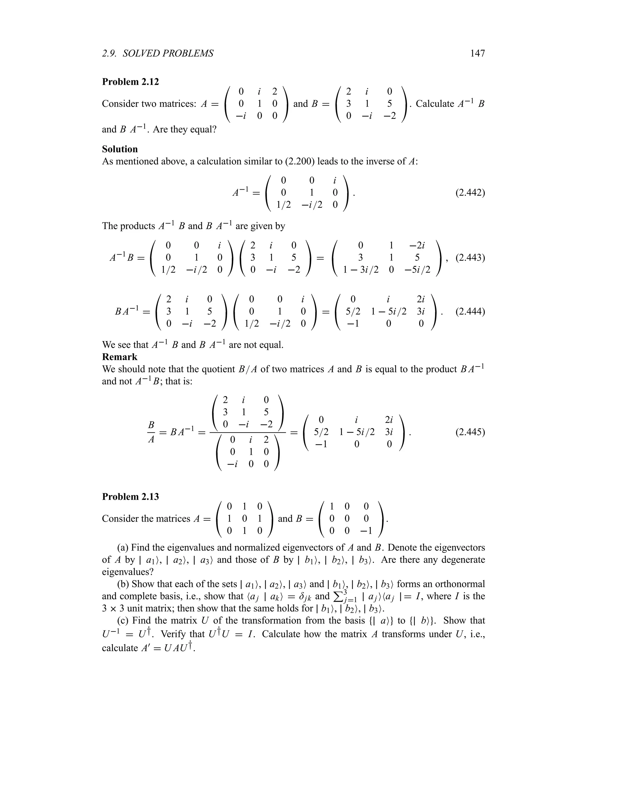
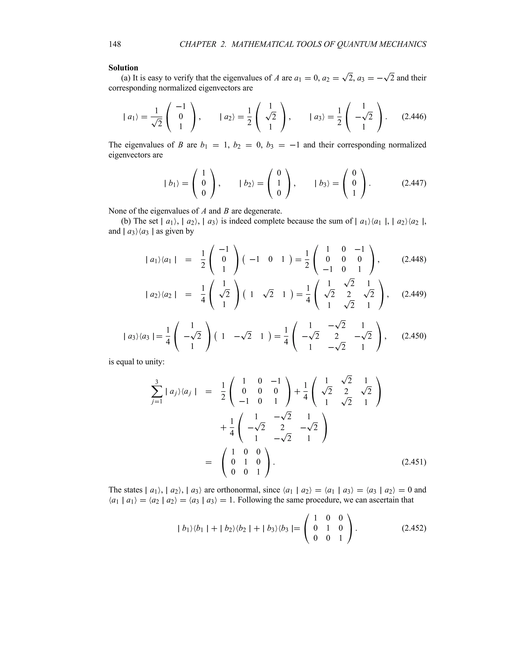
![150 CHAPTER 2. MATHEMATICAL TOOLS OF QUANTUM MECHANICS
Calculating the inverse of U as we did in (2.200), we see that it is equal to its Hermitian adjoint:
U1
1
2
#
T
2 0
T
2
1
T
2 1
1
T
2 1
$ U† (2.464)
This implies that the matrix U is unitary. The matrix A transforms as follows:
A)
U AU†
1
4
#
T
2 1 1
0
T
2
T
2
T
2 1 1
$
#
0 1 0
1 0 1
0 1 0
$
#
T
2 0
T
2
1
T
2 1
1
T
2 1
$
1
2
#
1
T
2 1 1
1 2 1
1 1 1
T
2
$ (2.465)
Problem 2.14
Calculate the following expressions involving Dirac’s delta function:
(a)
5 5
5 cos3x=x H3 dx
(b)
5 10
0
d
e2x7 4
e
=x 3 dx
(c)
d
2 cos23x sinx2
e
=x H
(d)
5 H
0 cos3A= )))A H2 dA
(e)
5 9
2
b
x2 5x 2
c
=[2x 4] dx.
Solution
(a) Since x H3 lies within the interval (5 5), equation (2.281) yields
= 5
5
cos3x=x H3 dx cos
r
3
H
3
s
1 (2.466)
(b) Since x 3 lies outside the interval (0 10), Eq (2.281) yields at once
= 10
0
K
e2x7
4
L
=x 3 dx 0 (2.467)
(c) Using the relation f x=x a f a=x a which is listed in Appendix A, we
have
K
2 cos2
3x sinx2
L
=x H
K
2 cos2
3H sinH2
L
=x H
3=x H (2.468)
(d) Inserting n 3 into Eq (2.282) and since cos)))3A 27 sin3A, we obtain
= H
0
cos3A= )))
A H2 dA 13
cos)))
3H2 13
27 sin3H2
27 (2.469)](https://image.slidesharecdn.com/zettili-250217213640-909f6141/75/Zettili-Quantum-mechanics-Concept-and-application-pdf-167-2048.jpg)
![2.9. SOLVED PROBLEMS 151
(e) Since =[2x 4] 12=x 4, we have
= 9
2
r
x2
5x 2
s
=[2x 4] dx
1
2
= 9
2
r
x2
5x 2
s
=x 4 dx
1
2
r
42
5 4 2
s
1 (2.470)
Problem 2.15
Consider a system whose Hamiltonian is given by H : M1ONM2 M2ONM1 , where : is
a real number having the dimensions of energy and M1O, M2O are normalized eigenstates of a
Hermitian operator A that has no degenerate eigenvalues.
(a) Is H a projection operator? What about :2 H2?
(b) Show that M1O and M2O are not eigenstates of H.
(c) Calculate the commutators [H M1ONM1 ] and [H M2ONM2 ] then find the relation
that may exist between them.
(d) Find the normalized eigenstates of H and their corresponding energy eigenvalues.
(e) Assuming that M1O and M2O form a complete and orthonormal basis, find the matrix
representing H in the basis. Find the eigenvalues and eigenvectors of the matrix and compare
the results with those derived in (d).
Solution
(a) Since M1O and M2O are eigenstates of A and since A is Hermitian, they must be
orthogonal, NM1 M2O 0 (instance of Theorem 2.1). Now, since M1O and M2O are both
normalized and since NM1 M2O 0, we can reduce H2 to
H2
:2
M1ONM2 M2ONM1 M1ONM1 M2ONM2
:2
M1ONM2 M2ONM1 (2.471)
which is different from H; hence H is not a projection operator. The operator :2 H2 is a
projection operator since it is both Hermitian and equal to its own square. Using (2.471) we
can write
:2
H2
2
M1ONM2 M2ONM1 M1ONM2 M2ONM1
M1ONM1 M2ONM2 :2
H2
(2.472)
(b) Since M1O and M2O are both normalized, and since NM1 M2O 0, we have
H M1O : M1ONM2 M1O : M2ONM1 M1O : M2O (2.473)
H M2O : M1O (2.474)
hence M1O and M2O are not eigenstates of H. In addition, we have
NM1 H M1O NM2 H M2O 0 (2.475)
(c) Using the relations derived above, H M1O : M2O and H M2O : M1O, we can
write
[H M1ONM1 ] : M2ONM1 M1ONM2 (2.476)](https://image.slidesharecdn.com/zettili-250217213640-909f6141/75/Zettili-Quantum-mechanics-Concept-and-application-pdf-168-2048.jpg)
![152 CHAPTER 2. MATHEMATICAL TOOLS OF QUANTUM MECHANICS
[H M2ONM2 ] : M1ONM2 M2ONM1 (2.477)
hence
[H M1ONM1 ] [H M2ONM2 ] (2.478)
(d) Consider a general state OO D1 M1O D2 M2O. Applying H to this state, we get
H OO : M1ONM2 M2ONM1 D1 M1O D2 M2O
: D2 M1O D1 M2O (2.479)
Now, since OO is normalized, we have
NO OO D1
2
D2
2
1 (2.480)
The previous two equations show that D1 D2 1
T
2 and that D1 D2. Hence the
eigenstates of the system are:
OO
1
T
2
M1O M2O (2.481)
The corresponding eigenvalues are ::
H OO : OO (2.482)
(e) Since NM1 M2O NM2 M1O 0 and NM1 M1O NM2 M2O 1, we can verify
that H11 NM1 H M1O 0, H22 NM2 H M2O 0, H12 NM1 H M2O :,
H21 NM2 H M1O :. The matrix of H is thus given by
H :
t
0 1
1 0
u
(2.483)
The eigenvalues of this matrix are equal to : and the corresponding eigenvectors are 1
T
2
t
1
1
u
.
These results are indeed similar to those derived in (d).
Problem 2.16
Consider the matrices A
#
1 0 0
0 7 3i
0 3i 5
$ and B
#
0 i 3i
i 0 i
3i i 0
$.
(a) Check the hermiticity of A and B.
(b) Find the eigenvalues of A and B; denote the eigenvalues of A by a1, a2, and a3. Explain
why the eigenvalues of A are real and those of B are imaginary.
(c) Calculate TrA and detA. Verify TrA a1 a2 a3, detA a1a2a3.
Solution
(a) Matrix A is Hermitian but B is anti-Hermitian:
A†
#
1 0 0
0 7 3i
0 3i 5
$ A B†
#
0 i 3i
i 0 i
3i i 0
$ B (2.484)](https://image.slidesharecdn.com/zettili-250217213640-909f6141/75/Zettili-Quantum-mechanics-Concept-and-application-pdf-169-2048.jpg)
![2.10. EXERCISES 157
(c) Show that the products BB† and B†B are projection operators.
(d) Show that the operator BB† B†B is unitary.
(e) Consider C BB† B†B. Show that C M1O M1O and C M2O M2O.
Exercise 2.15
Prove the following two relations:
(a) eAeB eABe[AB]2,
(b) eA BeA B [A B] 1
2! [A [A B]] 1
3! [A [A [A B]]] .
Hint: To prove the first relation, you may consider defining an operator function Ft eAt eBt,
where t is a parameter, A and B are t-independent operators, and then make use of [A GB]
[A B]dGBdB, where GB is a function depending on the operator B.
Exercise 2.16
(a) Verify that the matrix t
cos A sin A
sin A cos A
u
is unitary.
(b) Find its eigenvalues and the corresponding normalized eigenvectors.
Exercise 2.17
Consider the following three matrices:
A
#
0 1 0
1 0 1
0 1 0
$ B
#
0 i 0
i 0 i
0 i 0
$ C
#
1 0 0
0 0 0
0 0 1
$
(a) Calculate the commutators [A B], [B C], and [C A].
(b) Show that A2 B2 2C2 4I, where I is the unity matrix.
(c) Verify that TrABC TrBC A TrC AB.
Exercise 2.18
Consider the following two matrices:
A
#
3 i 1
1 i 2
4 3i 1
$ B
#
2i 5 3
i 3 0
7i 1 i
$
Verify the following relations:
(a) detAB detAdetB,
(b) detAT detA,
(c) detA† detA`
, and
(d) detA` detA`
.
Exercise 2.19
Consider the matrix
A
t
0 i
i 0
u
(a) Find the eigenvalues and the normalized eigenvectors for the matrix A.](https://image.slidesharecdn.com/zettili-250217213640-909f6141/75/Zettili-Quantum-mechanics-Concept-and-application-pdf-174-2048.jpg)

![2.10. EXERCISES 159
(c) Find the eigenvalues and eigenvectors of A and B.
(d) Are the eigenvectors of each operator orthonormal?
(e) Verify that U†BU is diagonal, U being the matrix of the normalized eigenvectors of B.
(f) Verify that U1 U†.
Exercise 2.25
Consider an operator A so that [A A
†
] 1.
(a) Evaluate the commutators [A
†
A A] and [A
†
A A
†
].
(b) If the actions of A and A
†
on the states aO are given by A aO
T
a a 1O and
A
†
aO
T
a 1 a 1O and if Na) aO =a)a, calculate Na A a 1O, Na 1 A
†
aO
and Na A
†
A aO and Na AA
†
aO.
(c) Calculate Na A A
†
2 aO and Na A A
†
2 aO.
Exercise 2.26
Consider a 4 4 matrix
A
%
%
#
0
T
1 0 0
0 0
T
2 0
0 0 0
T
3
0 0 0 0
$
(a) Find the matrices of A†, N A†A, H N 1
2 I (where I is the unit matrix), B
A A†, and C iA A†.
(b) Find the matrices corresponding to the commutators [A† A], [B C], [N B], and
[N C].
(c) Find the matrices corresponding to B2, C2, [N B2 C2], [H A†], [H A], and
[H N].
(d) Verify that detABC detAdetBdetC and detC† detC`
.
Exercise 2.27
If A and B commute, and if O1O and O2O are two eigenvectors of A with different eigenvalues
(A is Hermitian), show that
(a) NO1 B O2O is zero and
(b) B O1O is also an eigenvector to A with the same eigenvalue as O1O; i.e., if A O1O
a1 O1O, show that AB O1O a1 B O1O.
Exercise 2.28
Let A and B be two n n matrices. Assuming that B1 exists, show that [A B1]
B1[A B]B1.
Exercise 2.29
Consider a physical system whose Hamiltonian H and an operator A are given, in a three-
dimensional space, by the matrices
H
h
#
1 0 0
0 1 0
0 0 1
$ A a
#
1 0 0
0 0 1
0 1 0
$](https://image.slidesharecdn.com/zettili-250217213640-909f6141/75/Zettili-Quantum-mechanics-Concept-and-application-pdf-176-2048.jpg)
![160 CHAPTER 2. MATHEMATICAL TOOLS OF QUANTUM MECHANICS
(a) Are H and A Hermitian?
(b) Show that H and A commute. Give a basis of eigenvectors common to H and A.
Exercise 2.30
(a) Using [X P] i
h, show that [X2 P] 2i
hX and [X P2] 2i
hP.
(b) Show that [X2 P2] 2i
hi
h 2P X.
(c) Calculate the commutator [X2 P3].
Exercise 2.31
Discuss the hermiticity of the commutators [X P], [X2 P] and [X P2].
Exercise 2.32
(a) Evaluate the commutator [X2 ddx] by operating it on a wave function.
(b) Using [X P] i
h, evaluate the commutator [X P2 P X2] in terms of a linear combi-
nation of X2 P2 and X P.
Exercise 2.33
Show that [X Pn] i
hX Pn1.
Exercise 2.34
Evaluate the commutators [ei X P], [ei X2
P], and [ei X P2].
Exercise 2.35
Consider the matrix
A
#
0 0 1
0 1 0
1 0 0
$
(a) Find the eigenvalues and the normalized eigenvectors of A.
(b) Do these eigenvectors form a basis (i.e., is this basis complete and orthonormal)?
(c) Consider the matrix U which is formed from the normalized eigenvectors of A. Verify
that U is unitary and that it satisfies the relation
U†AU
#
D1 0 0
0 D2 0
0 0 D3
$
where D1, D2, and D3 are the eigenvalues of A.
(d) Show that ex A cosh x A sinh x.
Hint: cosh x
3*
n0 x2n2n! and sinh x
3*
n0 x2n12n 1!.
Exercise 2.36
(a) If [A B] c, where c is a number, prove the following two relations: eA BeA B c
and eAB eAeBec2.
(b) Now if [A B] cB, where c is again a number, show that eA BeA ec B.
Exercise 2.37
Consider the matrix
A
1
2
#
2 0 0
0 3 1
0 1 3
$](https://image.slidesharecdn.com/zettili-250217213640-909f6141/75/Zettili-Quantum-mechanics-Concept-and-application-pdf-177-2048.jpg)
![162 CHAPTER 2. MATHEMATICAL TOOLS OF QUANTUM MECHANICS
Exercise 2.44
Use the relations listed in Appendix A to evaluate the following integrals involving Dirac’s
delta function:
(a)
5 H
0 sin3x cos24x=x H2 dx.
(b)
5 2
2 e7x2=5x dx.
(c)
5 2H
2H sinA2= ))A H dA.
(d)
5 2H
0 cos2 A=[A H4] dA.
Exercise 2.45
Use the relations listed in Appendix A to evaluate the following expressions:
(a)
5 5
0 3x2 2=x 1 dx.
(b) 2x5 4x3 1=x 2.
(c)
5 *
0 5x3 7x2 3= x2 4 dx.
Exercise 2.46
Use the relations listed in Appendix A to evaluate the following expressions:
(a)
5 7
3 e6x2=4x dx.
(b) cos2A sinA=A2 H24.
(c)
5 1
1 e5x1= )))x dx.
Exercise 2.47
If the position and momentum operators are denoted by ;
R and ;
P, respectively, show that
P† ;
R nP 1n ;
R n and P† ;
P nP 1n ;
P n, where P is the parity operator and n is
an integer.
Exercise 2.48
Consider an operator
A M1ONM1 M2ONM2 M3ONM3 i M1ONM2
M1ONM3 i M2ONM1 M3ONM1
where M1O, M2O, and M3O form a complete and orthonormal basis.
(a) Is A Hermitian? Calculate A
2
; is it a projection operator?
(b) Find the 3 3 matrix representing A in the M1O, M2O, M3O basis.
(c) Find the eigenvalues and the eigenvectors of the matrix.
Exercise 2.49
The Hamiltonian of a two-state system is given by
H E M1ONM1 M2ONM2 i M1ONM2 i M2ONM1
where M1O, M2O form a complete and orthonormal basis; E is a real constant having the
dimensions of energy.
(a) Is H Hermitian? Calculate the trace of H.
(b) Find the matrix representing H in the M1O, M2O basis and calculate the eigenvalues
and the eigenvectors of the matrix. Calculate the trace of the matrix and compare it with the
result you obtained in (a).
(c) Calculate [H M1ONM1 ], [H M2ONM2 ], and [H M1ONM2 ].](https://image.slidesharecdn.com/zettili-250217213640-909f6141/75/Zettili-Quantum-mechanics-Concept-and-application-pdf-179-2048.jpg)
![2.10. EXERCISES 163
Exercise 2.50
Consider a particle which is confined to move along the positive x-axis and whose Hamiltonian
is H Ed2dx2, where E is a positive real constant having the dimensions of energy.
(a) Find the wave function that corresponds to an energy eigenvalue of 9E (make sure that
the function you find is finite everywhere along the positive x-axis and is square integrable).
Normalize this wave function.
(b) Calculate the probability of finding the particle in the region 0 n x n 15.
(c) Is the wave function derived in (a) an eigenfunction of the operator A ddx 7?
(d) Calculate the commutator [H A].
Exercise 2.51
Consider the wave functions:
Ox y sin 2x cos 5x Mx y e2x2y2
Nx y eixy
(a) Verify if any of the wave functions is an eigenfunction of A x y.
(b) Find out if any of the wave functions is an eigenfunction of B 2x2 2y2 1.
(c) Calculate the actions of AB and B A on each one of the wave functions and infer [A B].
Exercise 2.52
(a) Is the state OA M e3iM cos A an eigenfunction of AM M or of BA A?
(b) Are AM and BA Hermitian?
(c) Evaluate the expressions NO AM OO and NO BA OO.
(d) Find the commutator [AM BA ].
Exercise 2.53
Consider an operator A Xddx 2.
(a) Find the eigenfunction of A corresponding to a zero eigenvalue. Is this function normal-
izable?
(b) Is the operator A Hermitian?
(c) Calculate [A X], [A ddx], [A d2dx2], [X [A X]], and [ddx [A ddx]].
Exercise 2.54
If A and B are two Hermitian operators, find their respective eigenvalues such that A
2
2I
and B4 I, where I is the unit operator.
Exercise 2.55
Consider the Hilbert space of two-variable complex functions Ox y. A permutation operator
is defined by its action on Ox y as follows: HOx y Oy x.
(a) Verify that the operator H is linear and Hermitian.
(b) Show that H2 I. Find the eigenvalues and show that the eigenfunctions of H are given
by
Ox y
1
2
d
Ox y Oy x
e
and Ox y
1
2
d
Ox y Oy x
e](https://image.slidesharecdn.com/zettili-250217213640-909f6141/75/Zettili-Quantum-mechanics-Concept-and-application-pdf-180-2048.jpg)


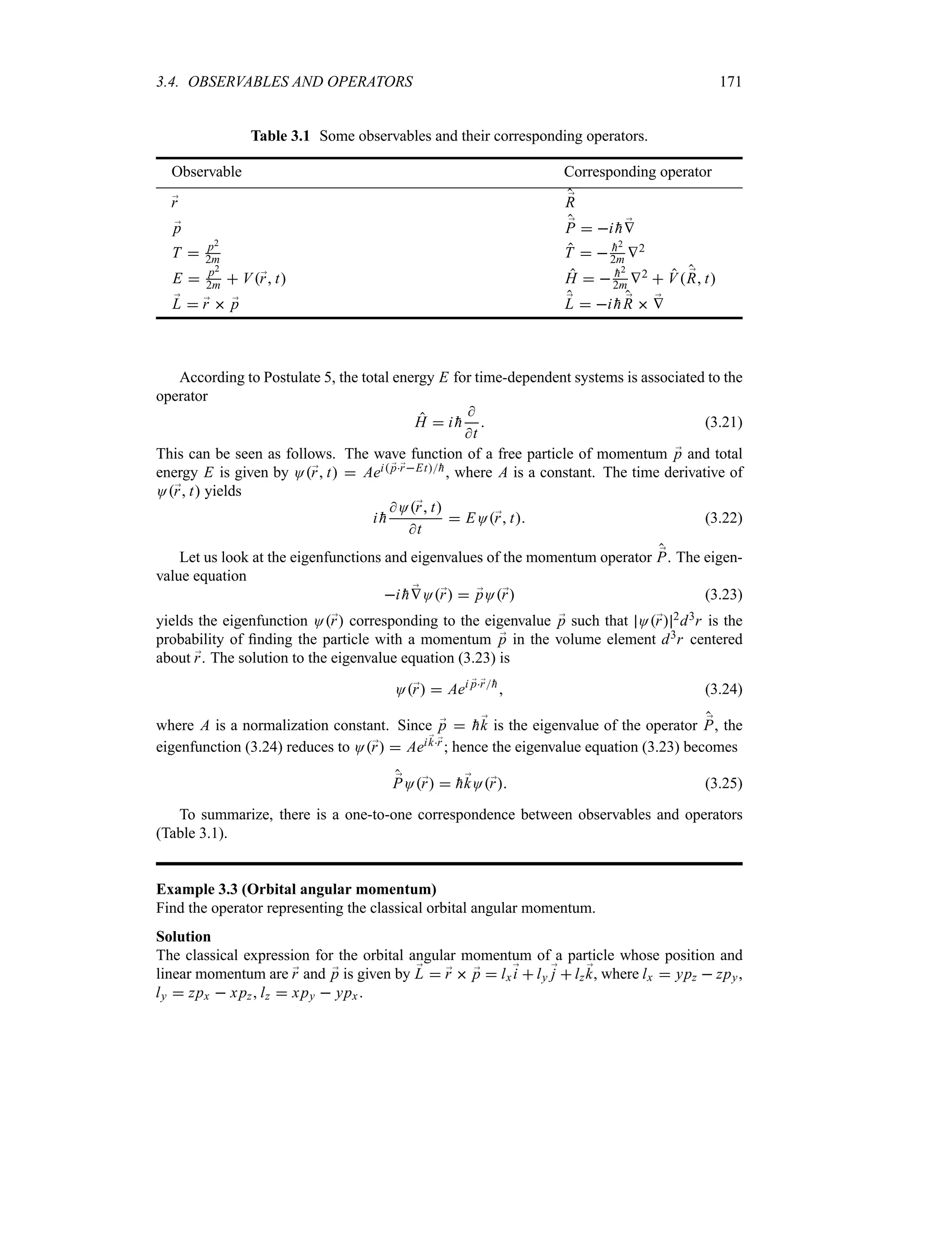


![3.5. MEASUREMENT IN QUANTUM MECHANICS 175
P3E3
NM3 OO 2
NO OO
n
n
n
n
n
U
2
19
NM3 M3O
n
n
n
n
n
2
19
15
2
15
(3.39)
P4E4
NM4 OO 2
NO OO
n
n
n
n
n
U
3
19
NM4 M4O
n
n
n
n
n
2
19
15
3
15
(3.40)
and
P5E5
NM5 OO 2
NO OO
n
n
n
n
n
U
5
19
NM5 M5O
n
n
n
n
n
2
19
15
5
15
(3.41)
(b) The average energy of a system is given by
E
5
;
j1
Pj E j
1
15
0
8
15
0
6
15
0
12
15
0
25
15
0
52
15
0 (3.42)
This energy can also be obtained from the expectation value of the Hamiltonian:
E
NO H OO
NO OO
19
15
5
;
n1
a2
nNMn H MnO
19
15
t
1
19
8
19
6
19
12
19
25
19
u
0
52
15
0 (3.43)
where the values of the coefficients a2
n are listed in (3.36).
3.5.3 Complete Sets of Commuting Operators (CSCO)
Two observables A and B are said to be compatible when their corresponding operators com-
mute, [A B] 0; observables corresponding to noncommuting operators are said to be non-
compatible.
In what follows we are going to consider the task of measuring two observables A and B
on a given system. Since the act of measurement generally perturbs the system, the result of
measuring A and B therefore depends on the order in which they are carried out. Measuring A
first and then B leads2 in general to results that are different from those obtained by measuring
B first and then A. How does this take place?
If A and B do not commute and if the system is in an eigenstate Oa
n O of A, a measurement
of A yields with certainty a value an, since A Oa
n O an Oa
n O. Then, when we measure B, the
state of the system will be left in one of the eigenstates of B. If we measure A again, we will
find a value which will be different from an. What is this new value? We cannot answer this
question with certainty: only a probabilistic outcome is possible. For this, we need to expand
the eigenstates of B in terms of those of A, and thus provide a probabilistic answer as to the
value of measuring A. So if A and B do not commute, they cannot be measured simultaneously;
the order in which they are measured matters.
2The act of measuring A first and then B is represented by the action of product B A of their corresponding operators
on the state vector.](https://image.slidesharecdn.com/zettili-250217213640-909f6141/75/Zettili-Quantum-mechanics-Concept-and-application-pdf-192-2048.jpg)
![176 CHAPTER 3. POSTULATES OF QUANTUM MECHANICS
What happens when A and B commute? We can show that the results of their measurements
will not depend on the order in which they are carried out. Before showing this, let us mention
a useful theorem.
Theorem 3.1 If two observables are compatible, their corresponding operators possess a set
of common (or simultaneous) eigenstates (this theorem holds for both degenerate and nonde-
generate eigenstates).
Proof
We provide here a proof for the nondegenerate case only. If OnO is a nondegenerate eigenstate
of A, A OnO an OnO, we have
NOm [A B] OnO am anNOm B OnO 0 (3.44)
since A and B commute. So NOm B OnO must vanish unless an am. That is,
NOm B OnO NOn B OnO ( =nm (3.45)
Hence the OnO are joint or simultaneous eigenstates of A and B (this completes the proof).
Denoting the simultaneous eigenstate of A and B by Oa
n1 Ob
n2 O, we have
A Oa
n1
Ob
n2
O an1 Oa
n1
Ob
n2
O (3.46)
B Oa
n1
Ob
n2
O bn2 Oa
n1
Ob
n2
O (3.47)
Theorem 3.1 can be generalized to the case of many mutually compatible observables A,
B, C, . These compatible observables possess a complete set of joint eigenstates
OnO Oa
n1
Ob
n2
Oc
n3
O (3.48)
The completeness and orthonormality conditions of this set are
;
n1
;
n2
;
n3
Oa
n1
Ob
n2
Oc
n3
ONOa
n1
Ob
n2
Oc
n3
1 (3.49)
NOn) OnO =n)n =n1
)n1 =n2
)n2 =n3
)n3 (3.50)
Let us now show why, when two observables A and B are compatible, the order in which
we carry out their measurements is irrelevant. Measuring A first, we would find a value an
and would leave the system in an eigenstate of A. According to Theorem 3.1, this eigenstate is
also an eigenstate of B. Thus a measurement of B yields with certainty bn without affecting the
state of the system. In this way, if we measure A again, we obtain with certainty the same initial
value an. Similarly, another measurement of B will yield bn and will leave the system in the
same joint eigenstate of A and B. Thus, if two observables A and B are compatible, and if the
system is initially in an eigenstate of one of their operators, their measurements not only yield
precise values (eigenvalues) but they will not depend on the order in which the measurements
were performed. In this case, A and B are said to be simultaneously measurable. So com-
patible observables can be measured simultaneously with arbitrary accuracy; noncompatible
observables cannot.
What happens if an operator, say A, has degenerate eigenvalues? The specification of
one eigenvalue does not uniquely determine the state of the system. Among the degenerate](https://image.slidesharecdn.com/zettili-250217213640-909f6141/75/Zettili-Quantum-mechanics-Concept-and-application-pdf-193-2048.jpg)
![3.5. MEASUREMENT IN QUANTUM MECHANICS 177
eigenstates of A, only a subset of them are also eigenstates of B. Thus, the set of states that
are joint eigenstates of both A and B is not complete. To resolve the degeneracy, we can
introduce a third operator C which commutes with both A and B; then we can construct a set of
joint eigenstates of A, B, and C that is complete. If the degeneracy persists, we may introduce a
fourth operator D that commutes with the previous three and then look for their joint eigenstates
which form a complete set. Continuing in this way, we will ultimately exhaust all the operators
(that is, there are no more independent operators) which commute with each other. When that
happens, we have then obtained a complete set of commuting operators (CSCO). Only then will
the state of the system be specified unambiguously, for the joint eigenstates of the CSCO are
determined uniquely and will form a complete set (recall that a complete set of eigenvectors of
an operator is called a basis). We should, at this level, state the following definition.
Definition: A set of Hermitian operators, A, B, C, , is called a CSCO if the operators
mutually commute and if the set of their common eigenstates is complete and not degenerate
(i.e., unique).
The complete commuting set may sometimes consist of only one operator. Any operator
with nondegenerate eigenvalues constitutes, all by itself, a CSCO. For instance, the position
operator X of a one-dimensional, spinless particle provides a complete set. Its momentum
operator P is also a complete set; together, however, X and P cannot form a CSCO, for they
do not commute. In three-dimensional problems, the three-coordinate position operators X, Y,
and Z form a CSCO; similarly, the components of the momentum operator Px, Py, and Pz also
form a CSCO. In the case of spherically symmetric three-dimensional potentials, the set H,
;
L 2, Lz forms a CSCO. Note that in this case of spherical symmetry, we need three operators
to form a CSCO because H, ;
L 2, and Lz are all degenerate; hence the complete and unique
determination of the wave function cannot be achieved with one operator or with two.
In summary, when a given operator, say A, is degenerate, the wave function cannot be
determined uniquely unless we introduce one or more additional operators so as to form a
complete commuting set.
3.5.4 Measurement and the Uncertainty Relations
We have seen in Chapter 2 that the uncertainty condition pertaining to the measurement of any
two observables A and B is given by
AB o
1
2
N[A B]O (3.51)
where A
T
NA
2
O NAO2.
Let us illustrate this on the joint measurement of the position and momentum observables.
Since these observables are not compatible, their simultaneous measurement with infinite ac-
curacy is not possible; that is, since [X P] i
h there exists no state which is a simultaneous
eigenstate of X and P. For the case of the position and momentum operators, the relation (3.51)
yields
xp o
h
2
(3.52)
This condition shows that the position and momentum of a microscopic system cannot be mea-
sured with infinite accuracy both at once. If the position is measured with an uncertainty x,](https://image.slidesharecdn.com/zettili-250217213640-909f6141/75/Zettili-Quantum-mechanics-Concept-and-application-pdf-194-2048.jpg)
![178 CHAPTER 3. POSTULATES OF QUANTUM MECHANICS
the uncertainty associated with its momentum measurement cannot be smaller than
h2x.
This is due to the interference between the two measurements. If we measure the position first,
we perturb the system by changing its state to an eigenstate of the position operator; then the
measurement of the momentum throws the system into an eigenstate of the momentum operator.
Another interesting application of the uncertainty relation (3.51) is to the orbital angular
momentum of a particle. Since its components satisfy the commutator [Lx Ly] i
hLz, we
obtain
Lx Ly o
1
2
h NLzO (3.53)
We can obtain the other two inequalities by means of a cyclic permutation of x, y, and z. If
NLzO 0, Lx and Ly will have sharp values simultaneously. This occurs when the particle is in
an s state. In fact, when a particle is in an s state, we have NLx O NLyO NLzO 0; hence all
the components of orbital angular momentum will have sharp values simultaneously.
3.6 Time Evolution of the System’s State
3.6.1 Time Evolution Operator
We want to examine here how quantum states evolve in time. That is, given the initial state
Ot0O, how does one find the state OtO at any later time t? The two states can be related by
means of a linear operator Ut t0 such that
OtO Ut t0 Ot0O t t0 (3.54)
Ut t0 is known as the time evolution operator or propagator. From (3.54), we infer that
Ut0 t0 I (3.55)
where I is the unit (identity) operator.
The issue now is to find Ut t0. For this, we need simply to substitute (3.54) into the
time-dependent Schrödinger equation (3.5):
i
h
t
r
Ut t0 Ot0O
s
H
r
Ut t0 Ot0O
s
(3.56)
or
Ut t0
t
i
h
HUt t0 (3.57)
The integration of this differential equation depends on whether or not the Hamiltonian depends
on time. If it does not depend on time, and taking into account the initial condition (3.55), we
can easily ascertain that the integration of (3.57) leads to
Ut t0 eitt0H
h
and OtO eitt0H
h
Ot0O (3.58)
We will show in Section 3.7 that the operator Ut t0 eitt0H
h represents a finite time
translation.
If, on the other hand, H depends on time the integration of (3.57) becomes less trivial. We
will deal with this issue in Chapter 10 when we look at time-dependent potentials or at the](https://image.slidesharecdn.com/zettili-250217213640-909f6141/75/Zettili-Quantum-mechanics-Concept-and-application-pdf-195-2048.jpg)

![182 CHAPTER 3. POSTULATES OF QUANTUM MECHANICS
Multiplying both sides of (3.79) by `;
r t and both sides of (3.80) by ;
r t, and subtracting
the two resulting equations, we obtain
i
h
t
d
`
;
r t;
r t
e
h2
2m
K
`
;
r tV2
;
r t V2
`
L
(3.81)
We can rewrite this equation as
I;
r t
t
;
V ;
J 0 (3.82)
where I;
r t and ;
J are given by
I;
r t `
;
r t;
r t ;
J;
r t
i
h
2m
r
;
V`
` ;
V
s
(3.83)
I;
r t is called the probability density, while ;
J;
r t is the probability current density, or sim-
ply the current density, or even the particle density flux. By analogy with charge conservation
in electrodynamics, equation (3.82) is interpreted as the conservation of probability.
Let us find the relationship between the density operators It and It0. Since tO
Ut t0 t0O and Nt Nt0 U†t t0, we have
It tONt Ut t0 0ON0 U†t t0 (3.84)
This is known as the density operator for the state tO. Hence knowing It0 we can calcu-
late It as follows:
It Ut t0It0U†t t0 (3.85)
3.6.5 Time Evolution of Expectation Values
We want to look here at the time dependence of the expectation value of a linear operator; if the
state tO is normalized, the expectation value is given by
NAO Nt A tO (3.86)
Using (3.76) and (3.77), we can write dNAOdt as follows:
d
dt
NAO
1
i
h
Nt AH H A tO Nt
A
t
tO (3.87)
or
d
dt
NAO
1
i
h
N[A H]O N
A
t
O (3.88)
Two important results stem from this relation. First, if the observable A does not depend ex-
plicitly on time, the term At will vanish, so the rate of change of the expectation value of A
is given by N[A H]Oi
h. Second, besides not depending explicitly on time, if the observable A
commutes with the Hamiltonian, the quantity dNAOdt will then be zero; hence the expectation](https://image.slidesharecdn.com/zettili-250217213640-909f6141/75/Zettili-Quantum-mechanics-Concept-and-application-pdf-199-2048.jpg)
![3.7. SYMMETRIES AND CONSERVATION LAWS 183
value NAO will be constant in time. So if A commutes with the Hamiltonian and is not dependent
on time, the observable A is said to be a constant of the motion; that is, the expectation value of
an operator that does not depend on time and that commutes with the Hamiltonian is constant
in time:
If [H A] 0 and
A
t
0
dNAO
dt
0 NAO constant (3.89)
For instance, we can verify that the energy, the linear momentum, and the angular momentum
of an isolated system are conserved: dNHOdt 0, dN ;
POdt 0, and dN;
LOdt 0. This
implies that the expectation values of H, ;
P, and ;
L are constant. Recall from classical physics
that the conservation of energy, linear momentum, and angular momentum are consequences
of the following symmetries, respectively: homogeneity of time, homogeneity of space, and
isotropy of space. We will show in the following section that these symmetries are associated,
respectively, with invariances in time translation, space translation, and space rotation.
As an example, let us consider the time evolution of the expectation value of the den-
sity operator It tONt ; see (3.84). From (3.5), which leads to tOt
1i
hH tO and Nt t 1i
hNt H, we have
It
t
1
i
h
H tONt
1
i
h
tONt H
1
i
h
[It H] (3.90)
A substitution of this relation into (3.88) leads to
d
dt
NItO
1
i
h
N[It H]O N
It
t
O
1
i
h
N[It H]O
1
i
h
N[It H]O 0 (3.91)
So the density operator is a constant of the motion. In fact, we can easily show that
N[It H]O Nt [ tONt H] tO
Nt tONt H tO Nt H tONt tO
0 (3.92)
which, when combined with (3.90), yields NIttO 0.
Finally, we should note that the constants of motion are nothing but observables that can be
measured simultaneously with the energy to arbitrary accuracy. If a system has a complete set
of commuting operators (CSCO), the number of these operators is given by the total number of
constants of the motion.
3.7 Symmetries and Conservation Laws
We are interested here in symmetries that leave the Hamiltonian of an isolated system invariant.
We will show that for each such symmetry there corresponds an observable which is a constant
of the motion. The invariance principles relevant to our study are the time translation invariance
and the space translation invariance. We may recall from classical physics that whenever a
system is invariant under space translations, its total momentum is conserved; and whenever it
is invariant under rotations, its total angular momentum is also conserved.
To prepare the stage for symmetries and conservation laws in quantum mechanics, we are
going to examine the properties of infinitesimal and finite unitary transformations that are most
essential to these invariance principles.](https://image.slidesharecdn.com/zettili-250217213640-909f6141/75/Zettili-Quantum-mechanics-Concept-and-application-pdf-200-2048.jpg)
![184 CHAPTER 3. POSTULATES OF QUANTUM MECHANICS
3.7.1 Infinitesimal Unitary Transformations
In Chapter 2 we saw that the transformations of a state vector OO and an operator A under an
infinitesimal unitary transformation UG I iG are given by
O)
O I iG OO OO = OO (3.93)
A
)
I iGAI iG A i[G A] (3.94)
where and G are called the parameter and the generator of the transformation, respectively.
Let us consider two important applications of infinitesimal unitary transformations: time
and space translations.
3.7.1.1 Time Translations: G H
h
The application of U=t H I i
h=t H on a state OtO gives
t
I
i
h
=t H
u
OtO OtO
t
i
h
=t
u
H OtO (3.95)
Since H OtO i
h OtOt we have
t
I
i
h
=t H
u
OtO OtO =t
OtO
t
Ot =tO (3.96)
because OtO=t OtOt is nothing but the first-order Taylor expansion of Ot=tO. We
conclude from (3.96) that the application of U=tH to OtO generates a state Ot=tO which
consists simply of a time translation of OtO by an amount equal to =t. The Hamiltonian in
I i
h=t H is thus the generator of infinitesimal time translations. Note that this translation
preserves the shape of the state OtO, for its overall shape is merely translated in time by =t.
3.7.1.2 Spatial Translations: G Px
h
The application of UPx I i
hPx to Ox gives
t
I
i
h
Px
u
Ox Ox
t
i
h
u
Px Ox (3.97)
Since Px i
hx and since the first-order Taylor expansion of Ox is given by
Ox Ox Oxx, we have
t
I
i
h
Px
u
Ox Ox
Ox
x
Ox (3.98)
So, when UPx acts on a wave function, it translates it spatially by an amount equal to .
Using [X Px ] i
h we infer from (3.94) that the position operator X transforms as follows:
X)
t
I
i
h
Px
u
X
t
I
i
h
Px
u
X
i
h
[Px X] X (3.99)
The relations (3.98) and (3.99) show that the linear momentum operator in I i
hPx is a
generator of infinitesimal spatial translations.](https://image.slidesharecdn.com/zettili-250217213640-909f6141/75/Zettili-Quantum-mechanics-Concept-and-application-pdf-201-2048.jpg)
![3.7. SYMMETRIES AND CONSERVATION LAWS 185
3.7.2 Finite Unitary Transformations
In Chapter 2 we saw that a finite unitary transformation can be constructed by performing a
succession of infinitesimal transformations. For instance, by applying a single infinitesimal
time translation N times in steps of KN, we can generate a finite time translation
UK H lim
N*
N
k1
t
I
i
h
K
N
H
u
lim
N*
t
I
i
h
K H
uN
exp
t
i
h
K H
u
(3.100)
where the Hamiltonian is the generator of finite time translations. We should note that the
time evolution operator Ut t0 eitt0H
h, displayed in (3.58), represents a finite unitary
transformation where H is the generator of the time translation.
By analogy with (3.96) we can show that the application of UK H to OtO yields
UK H OtO exp
t
i
h
K H
u
OtO Ot KO (3.101)
where Ot KO is merely a time translation of OtO.
Similarly, we can infer from (3.98) that the application of U;
a ;
P expi;
a ;
P
h to a wave
function causes it to be translated in space by a vector ;
a:
U;
a ;
PO;
r exp
t
i
h
;
a ;
P
u
O;
r O;
r ;
a (3.102)
To calculate the transformed position vector operator ;
R ), let us invoke a relation we derived
in Chapter 2:
A
)
ei:G
Aei:G
A i:[G A]
i:2
2!
[G [G A]]
i:3
3!
[G [G [G A]]]
(3.103)
An application of this relation to the spatial translation operator U;
a ;
P yields
;
R )
exp
t
i
h
;
a ;
P
u
;
R exp
t
i
h
;
a ;
P
u
;
R
i
h
[;
a ;
P ;
R] ;
R ;
a (3.104)
In deriving this, we have used the fact that [;
a ;
P ;
R] i
h;
a and that the other commutators
are zero, notably [;
a ;
P [;
a ;
P ;
R]] 0. From (3.102) and (3.104), we see that the linear
momentum in expi ;
a ;
P
h is a generator of finite spatial translations.
3.7.3 Symmetries and Conservation Laws
We want to show here that every invariance principle of H is connected with a conservation
law.
The Hamiltonian of a system transforms under a unitary transformation ei:G as follows;
see (3.103):
H)
ei:G
Hei:G
H i:[G H]
i:2
2!
[G [G H]]
i:3
3!
[G [G [G H]]]
(3.105)](https://image.slidesharecdn.com/zettili-250217213640-909f6141/75/Zettili-Quantum-mechanics-Concept-and-application-pdf-202-2048.jpg)
![186 CHAPTER 3. POSTULATES OF QUANTUM MECHANICS
If H commutes with G, it also commutes with the unitary transformation U:G ei:G.
In this case we may infer two important conclusions. On the one hand, there is an invariance
principle: the Hamiltonian is invariant under the transformation U:G, since
H)
ei:G
Hei:G
ei:G
ei:G
H H (3.106)
On the other hand, if in addition to [G H] 0, the operator G does not depend on time
explicitly, there is a conservation law: equation (3.88) shows that G is a constant of the motion,
since
d
dt
NGO
1
i
h
N[G H]O N
G
t
O 0 (3.107)
We say that G is conserved.
So whenever the Hamiltonian is invariant under a unitary transformation, the generator of
the transformation is conserved. We may say, in general, that for every invariance symmetry of
the Hamiltonian, there corresponds a conservation law.
3.7.3.1 Conservation of Energy and Linear Momentum
Let us consider two interesting applications pertaining to the invariance of the Hamiltonian
of an isolated system with respect to time translations and to space translations. First, let us
consider time translations. As shown in (3.58), time translations are generated in the case of
time-independent Hamiltonians by the evolution operator Ut t0 eitt0H
h. Since H
commutes with the generator of the time translation (which is given by H itself), it is invariant
under time translations. As H is invariant under time translations, the energy of an isolated
system is conserved. We should note that if the system is invariant under time translations,
this means there is a symmetry of time homogeneity. Time homogeneity implies that the time-
displaced state Ot K, like Ot, satisfies the Schrödinger equation.
The second application pertains to the spatial translations, or to transformations under
U;
a ;
P expi ;
a ;
P
h, of an isolated system. The linear momentum is invariant under U;
a ;
P
and the position operator transforms according to (3.104):
;
P )
;
P ;
R )
;
R ;
a (3.108)
For instance, since the Hamiltonian of a free particle does not depend on the coordinates, it
commutes with the linear momentum [H ;
P] 0. The Hamiltonian is then invariant under
spatial translations, since
H)
exp
t
i
h
;
a ;
P
u
H exp
t
i
h
;
a ;
P
u
exp
t
i
h
;
a ;
P
u
exp
t
i
h
;
a ;
P
u
H H (3.109)
Since [H ;
P] 0 and since the linear momentum operator does not depend explicitly on time,
we infer from (3.88) that ;
P is a constant of the motion, since
d
dt
N ;
PO
1
i
h
N[ ;
P H]O N
;
P
t
O 0 (3.110)
So if [H ;
P] 0 the Hamiltonian will be invariant under spatial translations and the linear
momentum will be conserved. A more general case where the linear momentum is a constant](https://image.slidesharecdn.com/zettili-250217213640-909f6141/75/Zettili-Quantum-mechanics-Concept-and-application-pdf-203-2048.jpg)
![3.8. CONNECTING QUANTUM TO CLASSICAL MECHANICS 187
of the motion is provided by an isolated system, for its total linear momentum is conserved.
Note that the invariance of the system under spatial translations means there is a symmetry of
spatial homogeneity. The requirement for the homogeneity of space implies that the spatially
displaced wave function O;
r ;
a, much like O;
r, satisfies the Schrödinger equation.
In summary, the symmetry of time homogeneity gives rise to the conservation of energy,
whereas the symmetry of space homogeneity gives rise to the conservation of linear momentum.
In Chapter 7 we will see that the symmetry of space isotropy, or the invariance of the
Hamiltonian with respect to space rotations, leads to conservation of the angular momentum.
Parity operator
The unitary transformations we have considered so far, time translations and space translations,
are continuous. We may consider now a discrete unitary transformation, the parity. As seen in
Chapter 2, the parity transformation consists of an inversion or reflection through the origin of
the coordinate system:
PO;
r O;
r (3.111)
If the parity operator commutes with the system’s Hamiltonian,
[H P] 0 (3.112)
the parity will be conserved, and hence a constant of the motion. In this case the Hamiltonian
and the parity operator have simultaneous eigenstates. For instance, we will see in Chapter 4
that the wave functions of a particle moving in a symmetric potential, V;
r V;
r, have
definite parities: they can be only even or odd. Similarly, we can ascertain that the parity of an
isolated system is a constant of the motion.
3.8 Connecting Quantum to Classical Mechanics
3.8.1 Poisson Brackets and Commutators
To establish a connection between quantum mechanics and classical mechanics, we may look
at the time evolution of observables.
Before describing the time evolution of a dynamical variable within the context of classical
mechanics, let us review the main ideas of the mathematical tool relevant to this description,
the Poisson bracket. The Poisson bracket between two dynamical variables A and B is defined
in terms of the generalized coordinates qi and the momenta pi of the system:
A B
;
j
t
A
qj
B
pj
A
pj
B
qj
u
(3.113)
Since the variables qi are independent of pi , we have qj pk 0, pj qk 0; thus we can
show that
qj qk pj pk 0 qj pk =jk (3.114)
Using (3.113) we can easily infer the following properties of the Poisson brackets:
Antisymmetry
A B B A (3.115)](https://image.slidesharecdn.com/zettili-250217213640-909f6141/75/Zettili-Quantum-mechanics-Concept-and-application-pdf-204-2048.jpg)
![188 CHAPTER 3. POSTULATES OF QUANTUM MECHANICS
Linearity
A :B ;C D : A B ; A C A D (3.116)
Complex conjugate
A B `
A`
B`
(3.117)
Distributivity
A BC A B C B A C AB C A B C A C B (3.118)
Jacobi identity
A B C B C A C A B 0 (3.119)
Using d f nxdx nf n1xd f xdx, we can show that
A Bn
nBn1
A B An
B nAn1
A B (3.120)
These properties are similar to the properties of the quantum mechanical commutators seen in
Chapter 2.
The total time derivative of a dynamical variable A is given by
d A
dt
;
j
t
A
qj
qj
t
A
pj
pj
t
u
A
t
;
j
t
A
qj
H
pj
A
pj
H
pj
u
A
t
(3.121)
in deriving this relation we have used the Hamilton equations of classical mechanics:
dqj
dt
H
pj
dpj
dt
H
qj
(3.122)
where H is the Hamiltonian of the system. The total time evolution of a dynamical variable A
is thus given by the following equation of motion:
d A
dt
A H
A
t
(3.123)
Note that if A does not depend explicitly on time, its time evolution is given simply by d Adt
A H . If d Adt 0 or A H 0, A is said to be a constant of the motion.
Comparing the classical relation (3.123) with its quantum mechanical counterpart (3.88),
d
dt
NAO
1
i
h
N[A H]O N
A
t
O (3.124)
we see that they are identical only if we identify the Poisson bracket A H with the commuta-
tor [A H]i
h. We may thus infer the following general rule. The Poisson bracket of any pair
of classical variables can be obtained from the commutator between the corresponding pair of
quantum operators by dividing it by i
h:
1
i
h
[A B] A B classical (3.125)](https://image.slidesharecdn.com/zettili-250217213640-909f6141/75/Zettili-Quantum-mechanics-Concept-and-application-pdf-205-2048.jpg)
![3.8. CONNECTING QUANTUM TO CLASSICAL MECHANICS 189
Note that the expressions of classical mechanics can be derived from their quantum counter-
parts, but the opposite is not possible. That is, dividing quantum mechanical expressions by i
h
leads to their classical analog, but multiplying classical mechanical expressions by i
h doesn’t
necessarily lead to their quantum counterparts.
Example 3.5
(a) Evaluate the Poisson bracket x p between the position, x, and momentum, p, vari-
ables.
(b) Compare the commutator
K
X P
L
with Poisson bracket x p calculated in Part (a).
Solution
(a) Applying the general relation
A B
;
j
t
A
xj
B
pj
A
pj
B
x j
u
(3.126)
to x and p, we can readily evaluate the given Poisson bracket:
x p
x
x
p
p
x
p
p
x
x
x
p
p
1
(3.127)
(b) Using the fact that [X P] i
h , we see that
1
i
h
[ X P] 1 (3.128)
which is equal to the Poisson bracket (3.127); that is,
1
i
h
[ X P] x p classical 1 (3.129)
This result is in agreement with Eq. (3.125).
3.8.2 The Ehrenfest Theorem
If quantum mechanics is to be more general than classical mechanics, it must contain classical
mechanics as a limiting case. To illustrate this idea, let us look at the time evolution of the
expectation values of the position and momentum operators, ;
R and ;
P, of a particle moving in
a potential V;
r, and then compare these relations with their classical counterparts.
Since the position and the momentum observables do not depend explicitly on time, within
the context of wave mechanics, the terms N ;
RtO and N ;
PtO are zero. Hence, inserting](https://image.slidesharecdn.com/zettili-250217213640-909f6141/75/Zettili-Quantum-mechanics-Concept-and-application-pdf-206-2048.jpg)
![190 CHAPTER 3. POSTULATES OF QUANTUM MECHANICS
H ;
P 22m V ;
R t into (3.88) and using the fact that ;
R commutes with V ;
R t, we can
write
d
dt
N ;
RO
1
i
h
N[ ;
R H]O
1
i
h
N[ ;
R
;
P 2
2m
V ;
R t]O
1
2im
h
N[ ;
R ;
P 2
]O (3.130)
Since
[ ;
R ;
P 2
] 2i
h ;
P (3.131)
we have
d
dt
N ;
RO
1
m
N ;
PO (3.132)
As for dN ;
POdt, we can infer its expression from a treatment analogous to dN ;
ROdt. Using
[ ;
P V ;
R t] i
h ;
VV ;
R t (3.133)
we can write
d
dt
N ;
PO
1
i
h
N[ ;
P V ;
R t]O N ;
VV ;
R tO (3.134)
The two relations (3.132) and (3.134), expressing the time evolution of the expectation values
of the position and momentum operators, are known as the Ehrenfest theorem, or Ehrenfest
equations. Their respective forms are reminiscent of the Hamilton–Jacobi equations of classical
mechanics,
d;
r
dt
;
p
m
d ;
p
dt
;
VV;
r (3.135)
which reduce to Newton’s equation of motion for a classical particle of mass m, position ;
r, and
momentum ;
p:
d ;
p
dt
m
d2;
r
dt2
;
VV;
r (3.136)
Notice
h has completely disappeared in the Ehrenfest equations (3.132) and (3.134). These two
equations certainly establish a connection between quantum mechanics and classical mechan-
ics. We can, within this context, view the center of the wave packet as moving like a classical
particle when subject to a potential V;
r.
3.8.3 Quantum Mechanics and Classical Mechanics
In Chapter 1 we focused mainly on those experimental observations which confirm the failure
of classical physics at the microscopic level. We should bear in mind, however, that classical
physics works perfectly well within the realm of the macroscopic world. Thus, if the theory
of quantum mechanics is to be considered more general than classical physics, it must yield
accurate results not only on the microscopic scale but at the classical limit as well.
How does one decide on when to use classical or quantum mechanics to describe the motion
of a given system? That is, how do we know when a classical description is good enough or
when a quantum description becomes a must? The answer is provided by comparing the size of
those quantities of the system that have the dimensions of an action with the Planck constant,
h. Since, as shown in (3.125), the quantum relations are characterized by h, we can state that](https://image.slidesharecdn.com/zettili-250217213640-909f6141/75/Zettili-Quantum-mechanics-Concept-and-application-pdf-207-2048.jpg)
![3.9. SOLVED PROBLEMS 195
Now, taking the divergence of (3.161), we end up with
;
V ;
Jx t
d Jx t
dx
16H2
h
T
3
5ma3
sin
t
3Hx
a
u
sin
t
5Hx
a
u
sin
t
16E1t
h
u
(3.163)
The addition of (3.162) and (3.163) confirms the conservation of probability:
I
t
;
V ;
Jx t 0 (3.164)
Problem 3.3
Consider a one-dimensional particle which is confined within the region 0 n x n a and whose
wave function is x t sin Hxa expit.
(a) Find the potential Vx.
(b) Calculate the probability of finding the particle in the interval a4 n x n 3a4.
Solution
(a) Since the first time derivative and the second x derivative of x t are given by
x tt ix t and 2x tx2 H2a2x t, the Schrödinger equa-
tion (3.68) yields
i
hix t
h2
2m
H2
a2
x t Vx tx t (3.165)
Hence Vx t is time independent and given by Vx
h
h2H22ma2.
(b) The probability of finding the particle in the interval a4 n x n 3a4 can be obtained
from (3.4):
P
5 3a4
a4 Ox 2dx
5 a
0 Ox 2dx
5 3a4
a4 sin2
Hxa dx
5 a
0 sin2
Hxa dx
2 H
2H
082 (3.166)
Problem 3.4
A system is initially in the state O0O [
T
2 M1O
T
3 M2O M3O M4O]
T
7, where MnO are
eigenstates of the system’s Hamiltonian such that H MnO n2E0 MnO.
(a) If energy is measured, what values will be obtained and with what probabilities?
(b) Consider an operator A whose action on MnO is defined by A MnO n 1a0 MnO. If
A is measured, what values will be obtained and with what probabilities?
(c) Suppose that a measurement of the energy yields 4E0. If we measure A immediately
afterwards, what value will be obtained?
Solution
(a) A measurement of the energy yields En NMn H MnO n2E0, that is
E1 E0 E2 4E0 E3 9E0 E4 16E0 (3.167)
Since O0O is normalized, NO0 O0O 23117 1, and using (3.2), we can write the
probabilities corresponding to (3.167) as PEn NMn O0O 2
NO0 O0O NMn O0O 2
; hence,](https://image.slidesharecdn.com/zettili-250217213640-909f6141/75/Zettili-Quantum-mechanics-Concept-and-application-pdf-212-2048.jpg)
![196 CHAPTER 3. POSTULATES OF QUANTUM MECHANICS
using the fact that NMn MmO =nm, we have
PE1
n
n
n
n
n
U
2
7
NM1 M1O
n
n
n
n
n
2
2
7
PE2
n
n
n
n
n
U
3
7
NM2 M2O
n
n
n
n
n
2
3
7
(3.168)
PE3
n
n
n
n
1
T
7
NM3 M3O
n
n
n
n
2
1
7
PE4
n
n
n
n
1
T
7
NM4 M4O
n
n
n
n
2
1
7
(3.169)
(b) Similarly, a measurement of the observable A yields an NMn A MnO n 1a0; that
is,
a1 2a0 a2 3a0 a3 4a0 a4 5a0 (3.170)
Again, using (3.2) and since O0O is normalized, we can ascertain that the probabilities cor-
responding to the values (3.170) are given by Pan NMn O0O 2
NO0 O0O NMn O0O 2
,
or
Pa1
n
n
n
n
n
U
2
7
NM1 M1O
n
n
n
n
n
2
2
7
Pa2
n
n
n
n
n
U
3
7
NM2 M2O
n
n
n
n
n
2
3
7
(3.171)
Pa3
n
n
n
n
1
T
7
NM3 M3O
n
n
n
n
2
1
7
Pa4
n
n
n
n
1
T
7
NM4 M4O
n
n
n
n
2
1
7
(3.172)
(c) An energy measurement that yields 4E0 implies that the system is left in the state M2O.
A measurement of the observable A immediately afterwards leads to
NM2 A M2O 3a0NM2 M2O 3a0 (3.173)
Problem 3.5
(a) Assuming that the system of Problem 3.4 is initially in the state M3O, what values for the
energy and the observable A will be obtained if we measure: (i)H first then A, (ii) A first then
H?
(b) Compare the results obtained in (i) and (ii) and infer whether H and A are compatible.
Calculate [H A] M3O.
Solution
(a) (i) The measurement of H first then A is represented by AH M3O. Using the relations
H MnO n2E0 MnO and A MnO na0 Mn1O, we have
AH M3O 9E0 A M3O 27E0a0 M4O (3.174)
(ii) Measuring A first and then H, we will obtain
H A M3O 3a0 H M4O 48E0a0 M4O (3.175)
(b) Equations (3.174) and (3.175) show that the actions of AH and H A yield different
results. This means that H and A do not commute; hence they are not compatible. We can thus
write
[H A] M3O 48 27E0a0 M4O 17E0a0 M4O (3.176)](https://image.slidesharecdn.com/zettili-250217213640-909f6141/75/Zettili-Quantum-mechanics-Concept-and-application-pdf-213-2048.jpg)


![206 CHAPTER 3. POSTULATES OF QUANTUM MECHANICS
As expected, Et E0 since dNHOdt 0.
(d) Since none of the eigenvalues of H is degenerate, the eigenvectors M1O, M2O, M3O form
a compete (orthonormal) basis. Thus H forms a complete set of commuting operators.
Problem 3.12
(a) Calculate the Poisson bracket between the x and y components of the classical orbital
angular momentum.
(b) Calculate the commutator between the x and y components of the orbital angular mo-
mentum operator.
(c) Compare the results obtained in (a) and (b).
Solution
(a) Using the definition (3.113) we can write the Poisson bracket lx ly as
lxly
3
;
j1
t
lx
qj
ly
pj
lx
pj
ly
qj
u
(3.227)
where q1 x, q2 y, q3 z, p1 px , p2 py, and p3 pz. Since lx ypz zpy,
ly zpx xpz, lz xpy ypx , the only partial derivatives that survive are lx z py,
lypz x, lx pz y, and lyz px. Thus, we have
lx ly
lx
z
ly
pz
lx
pz
ly
z
xpy ypx lz (3.228)
(b) The components of ;
L are listed in (3.26) to (3.28): Lx Y Pz Z Py, Ly Z Px X Pz,
and LZ X Py Y Px. Since X, Y, and Z mutually commute and so do Px, Py, and Pz, we
have
[Lx Ly] [Y Pz Z Py Z Px X Pz]
[Y Pz Z Px ] [Y Pz X Pz] [Z Py Z Px ] [Z Py X Pz]
Y[Pz Z]Px X[Z Pz]Py i
hX Py Y Px
i
hLz (3.229)
(c) A comparison of (3.228) and (3.229) shows that
lxly lz [Lx Ly] i
hLz (3.230)
Problem 3.13
Consider a charged oscillator, of positive charge q and mass m, which is subject to an oscillating
electric field E0 cos t; the particle’s Hamiltonian is H P22m kX22 qE0 X cos t.
(a) Calculate dNXOdt, dNPOdt, dNHOdt.
(b) Solve the equation for dNXOdt and obtain NXOt such that NXO0 x0.
Solution](https://image.slidesharecdn.com/zettili-250217213640-909f6141/75/Zettili-Quantum-mechanics-Concept-and-application-pdf-223-2048.jpg)
![3.9. SOLVED PROBLEMS 207
(a) Since the position operator X does not depend explicitly on time (i.e., Xt 0),
equation (3.88) yields
d
dt
NXO
1
i
h
N[X H]O
1
i
h
N
v
X
P2
2m
w
O
NPO
m
(3.231)
Now, since [P X] i
h, [P X2] 2i
hX and Pt 0, we have
d
dt
NPO
1
i
h
N[P H]O
1
i
h
N
v
P
1
2
kX2
qE0 X cos t
w
O kNXO qE0 cos t
(3.232)
d
dt
NHO
1
i
h
N[H H]O N
H
t
O N
H
t
O qE0NXO sin t (3.233)
(b) To find NXO we need to take a time derivative of (3.231) and then make use of (3.232):
d2
dt2
NXO
1
m
d
dt
NPO
k
m
NXO
qE0
m
cos t (3.234)
The solution of this equation is
NXOt NXO0 cos
‚U
k
m
t
qE0
m
sin t A (3.235)
where A is a constant which can be determined from the initial conditions; since NXO0 x0
we have A 0, and hence
NXOt x0 cos
‚U
k
m
t
qE0
m
sin t (3.236)
Problem 3.14
Consider a one-dimensional free particle of mass m whose position and momentum at time
t 0 are given by x0 and p0, respectively.
(a) Calculate NPOt and show that NXOt p0t2m x0.
(b) Show that dNX2Odt 2NP XOm i
hm and dNP2Odt 0.
(c) Show that the position and momentum fluctuations are related by d2x2dt2
2p2m2 and that the solution to this equation is given by x2 p2
0t2m2 x2
0
where x0 and p0 are the initial fluctuations.
Solution
(a) From the Ehrenfest equations dNPOdt N[P Vx t]Oi
h as shown in (3.134), and
since for a free particle Vx t 0, we see that dNPOdt 0. As expected this leads to
NPOt p0, since the linear momentum of a free particle is conserved. Inserting NPO p0
into Ehrenfest’s other equation dNXOdt NPOm (see (3.132)), we obtain
dNXO
dt
1
m
p0 (3.237)](https://image.slidesharecdn.com/zettili-250217213640-909f6141/75/Zettili-Quantum-mechanics-Concept-and-application-pdf-224-2048.jpg)
![208 CHAPTER 3. POSTULATES OF QUANTUM MECHANICS
The solution of this equation with the initial condition NXO0 x0 is
NXOt
p0
m
t x0 (3.238)
(b) First, the proof of dNP2Odt 0 is straightforward. Since [P2 H] [P2 P22m] 0
and P2t 0 (the momentum operator does not depend on time), (3.124) yields
d
dt
NP2
O
1
i
h
N[P2
H]O N
P2
t
O 0 (3.239)
For dNX2Odt we have
d
dt
NX2
O
1
i
h
N[X2
H]O
1
2im
h
N[X2
P2
]O (3.240)
since X2t 0. Using [X P] i
h, we obtain
[X2
P2
] P[X2
P] [X2
P]P
PX[X P] P[X P]X X[X P]P [X P]X P
2i
hP X X P 2i
h2P X i
h (3.241)
hence
d
dt
NX2
O
2
m
NP XO
i
h
m
(3.242)
(c) As the position fluctuation is given by x2 NX2O NXO2, we have
dx2
dt
dNX2O
dt
2NXO
dNXO
dt
2
m
NP XO
i
h
m
2
m
NXONPO (3.243)
In deriving this expression we have used (3.242) and dNXOdt NPOm. Now, since
dNXONPOdt NPOdNXOdt NPO2m and
dNP XO
dt
1
i
h
N[P X H]O
1
2im
h
N[P X P2
]O
1
m
NP2
O (3.244)
we can write the second time derivative of (3.243) as follows:
d2x2
dt2
2
m
‚
dNP XO
dt
dNXONPO
dt
2
m2
r
NP2
O NPO2
s
2
m2
p2
0 (3.245)
where p2
0 NP2O NPO2 NP2O0 NPO2
0; the momentum of the free particle is a constant
of the motion. We can verify that the solution of the differential equation (3.245) is given by
x2
1
m2
p2
0t2
x2
0 (3.246)
This fluctuation is similar to the spreading of a Gaussian wave packet we derived in Chapter 1.](https://image.slidesharecdn.com/zettili-250217213640-909f6141/75/Zettili-Quantum-mechanics-Concept-and-application-pdf-225-2048.jpg)


![214 CHAPTER 3. POSTULATES OF QUANTUM MECHANICS
(c) Find the average value of the energy NHO and the energy uncertainty
T
NH2O NHO2.
(d) Find the state OtO.
Exercise 3.24
Prove the relation
d
dt
NABO N
A
t
BO NA
B
t
O
1
i
h
N[A H]BO
1
i
h
NA[B H]O
Exercise 3.25
Consider a particle of mass m which moves under the influence of gravity; the particle’s Hamil-
tonian is H P2
z 2m mgZ, where g is the acceleration due to gravity, g 98 m s2.
(a) Calculate dNZOdt, dNPzOdt, dNHOdt.
(b) Solve the equation dNZOdt and obtain NZOt, such that NZO0 h and NPzO0 0.
Compare the result with the classical relation zt 1
2 gt2 h.
Exercise 3.26
Calculate dNXOdt, dNPxOdt, dNHOdt for a particle with H P2
x 2m 1
2 m2 X2 V0 X3.
Exercise 3.27
Consider a system whose initial state at t 0 is given in terms of a complete and orthonormal
set of four vectors M1O, M2O, M3O, M4O as follows:
O0O
A
T
12
M1O
1
T
6
M2O
2
T
12
M3O
1
2
M4O
where A is a real constant.
(a) Find A so that O0O is normalized.
(b) If the energies corresponding to M1O, M2O, M3O, M4O are given by E1, E2, E3, and E4,
respectively, write down the state of the system OtO at any later time t.
(c) Determine the probability of finding the system at a time t in the state M2O.](https://image.slidesharecdn.com/zettili-250217213640-909f6141/75/Zettili-Quantum-mechanics-Concept-and-application-pdf-231-2048.jpg)
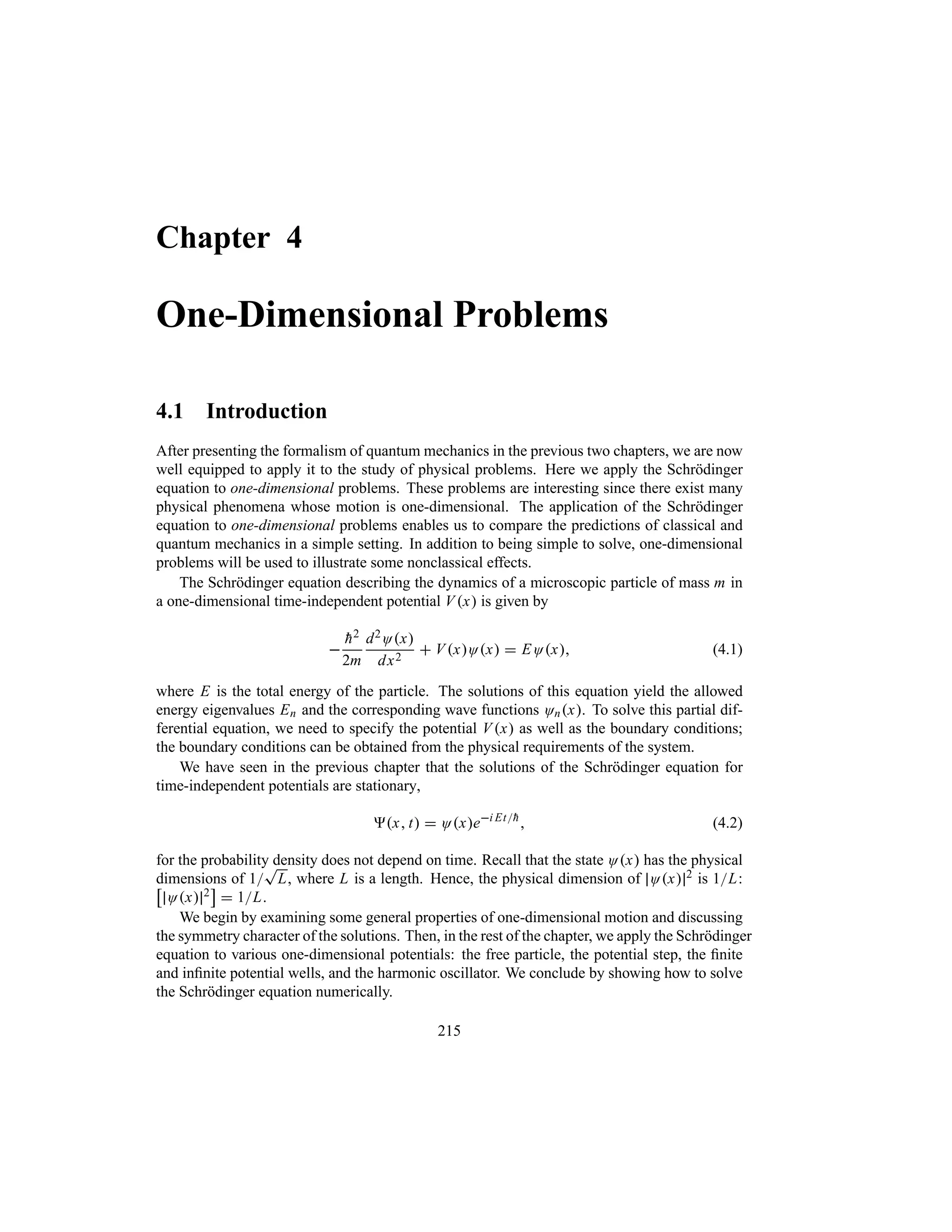
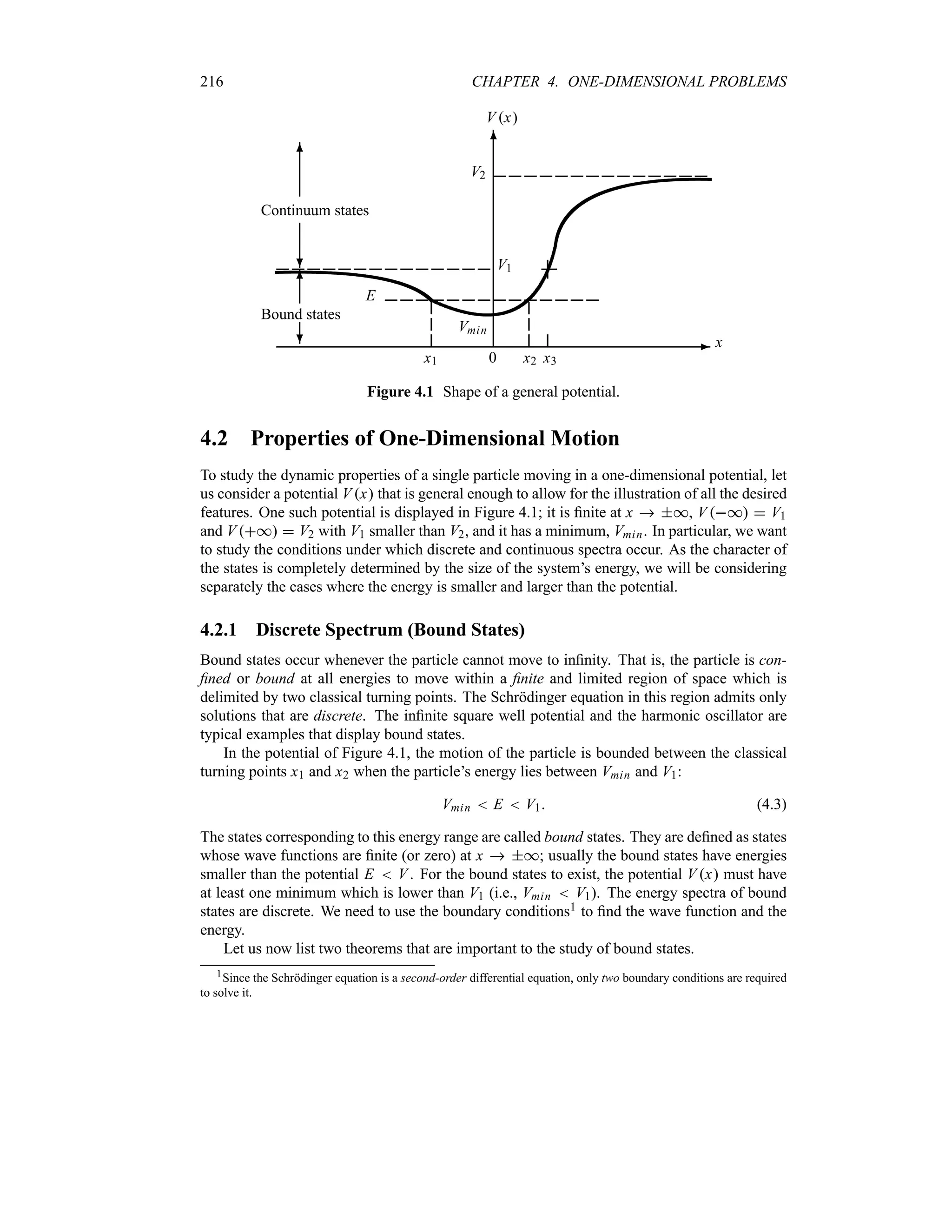

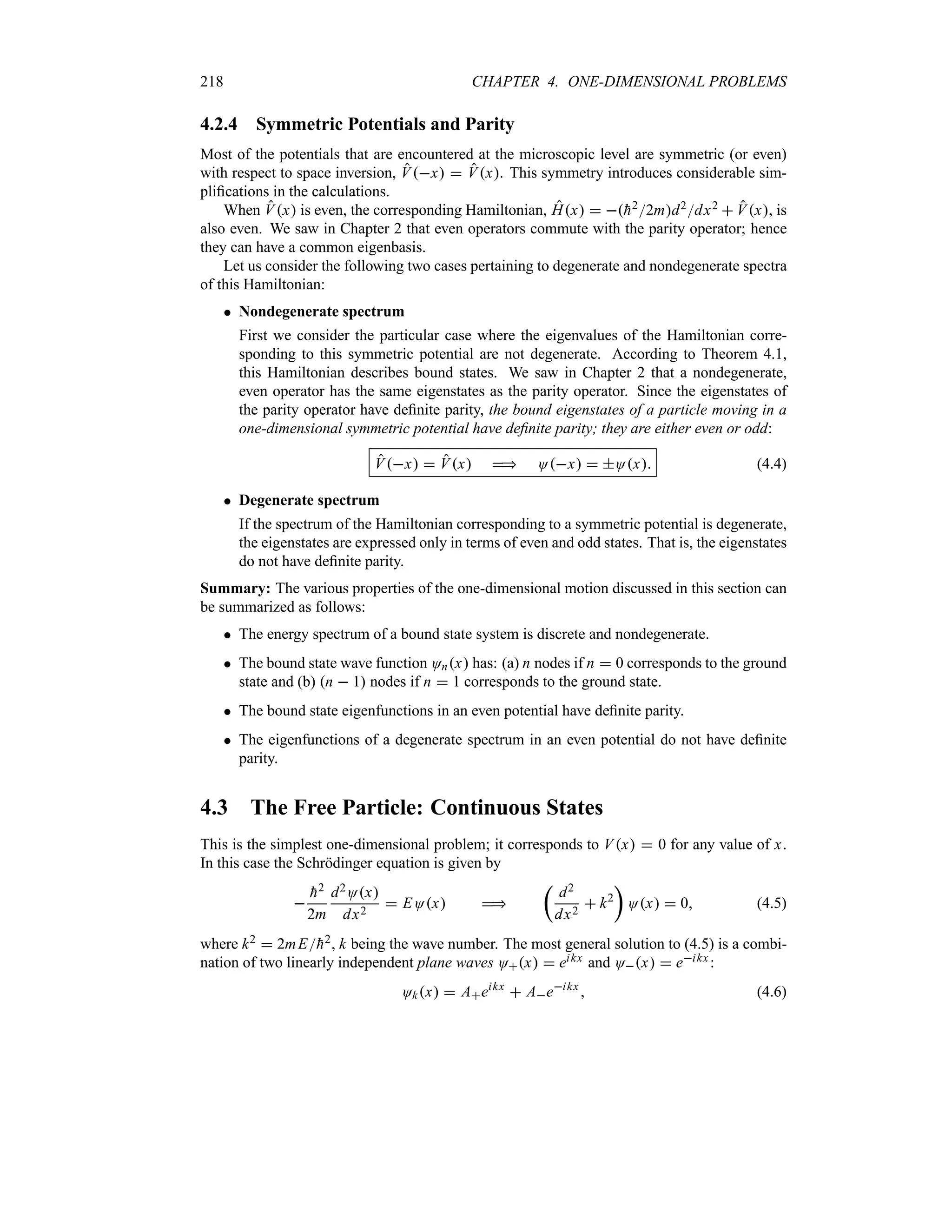
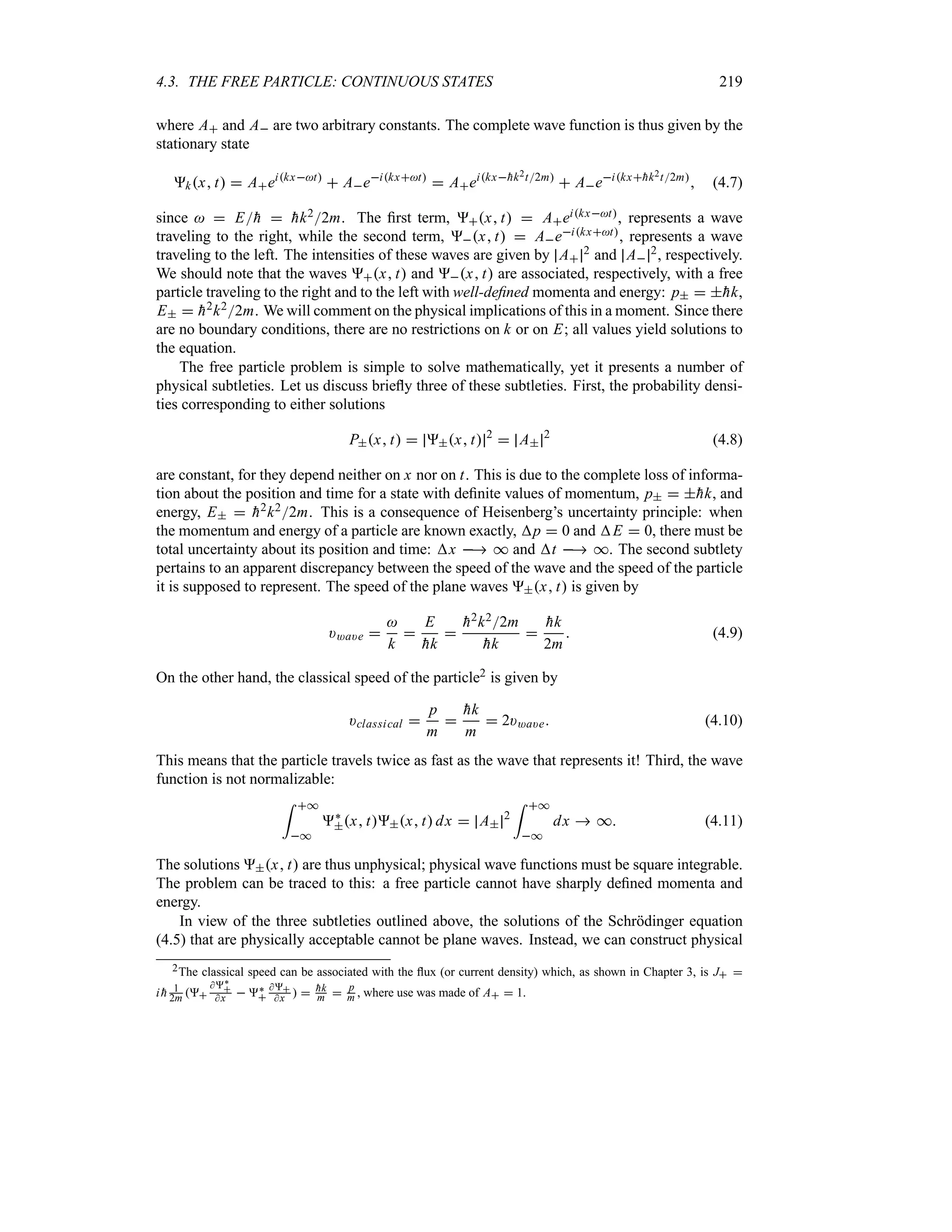
![4.4. THE POTENTIAL STEP 221
-
6
0
x
Ox 2
-
6
0
x
Ox 2
-
6
0
x
Vx
V0
E
Aeik1x
-
Beik1x
¾
Ceik2x
-
-
6
0
x
Vx
V0
Aeik1x
-
Beik1x
¾
Cek2x
E
D1 2Hk1
D2 2Hk2
E V0 E V0
Figure 4.2 Potential step and propagation directions of the incident, reflected, and transmitted
waves, plus their probability densities Ox 2
when E V0 and E V0.
t
d2
dx2
k2
2
u
O2x 0 x o 0 (4.16)
where k2
1 2mE
h2 and k2
2 2mE V0
h2. The most general solutions to these two
equations are plane waves:
O1x Aeik1x
Beik1x
x 0 (4.17)
O2x Ceik2x
Deik2x
x o 0 (4.18)
where Aeik1x and Ceik2x represent waves moving in the positive x-direction, but Beik1x and
Deik2x correspond to waves moving in the negative x-direction. We are interested in the case
where the particles are initially incident on the potential step from the left: they can be reflected
or transmitted at x 0. Since no wave is reflected from the region x 0 to the left, the constant
D must vanish. Since we are dealing with stationary states, the complete wave function is thus
given by
x t
|
O1xeit Aeik1xt Beik1xt x 0
O2xeit Ceik2xt x o 0
(4.19)
where A exp[ik1x t], B exp[ik1x t], and C exp[ik2x t] represent the incident,
the reflected, and the transmitted waves, respectively; they travel to the right, the left, and the
right (Figure 4.2). Note that the probability density Ox 2
shown in the lower left plot of
Figure 4.2 is a straight line for x 0, since O2x 2
C exp ik2x t 2
C 2
.
Let us now evaluate the reflection and transmission coefficients, R and T, as defined by
R
n
n
n
n
reflected current density
incident current density
n
n
n
n
n
n
n
n
Jref lected
Jincident
n
n
n
n T
n
n
n
n
Jtransmitted
Jincident
n
n
n
n (4.20)](https://image.slidesharecdn.com/zettili-250217213640-909f6141/75/Zettili-Quantum-mechanics-Concept-and-application-pdf-238-2048.jpg)
![4.5. THE POTENTIAL BARRIER AND WELL 225
-
6
0 a
x
Ox 2
E V0
-
6
0 a
x
Ox 2
E V0
-
6
0 a
x
Vx
V0
Aeik1x
-
Beik1x
¾
Ceik2x
-
Deik2x
¾
Eeik1x
-
E
-
6
0 a
x
Vx
V0
Aeik1x
-
Beik1x
¾
Dek2x
Cek2x
Eeik1x
-
E
Figure 4.3 Potential barrier and propagation directions of the incident, reflected, and transmit-
ted waves, plus their probability densities Ox 2 when E V0 and E V0.
O10 O20
dO10
dx
dO20
dx
(4.37)
O2a O3a
dO2a
dx
dO3a
dx
(4.38)
These equations yield
A B C D ik1A B ik2C D (4.39)
Ceik2a
Deik2a
Eeik1a
ik2
r
Ceik2a
Deik2a
s
ik1Eeik1a
(4.40)
Solving for E, we obtain
E 4k1k2 Aeik1a
[k1 k22
eik2a
k1 k22
eik2a
]1
4k1k2 Aeik1a
K
4k1k2 cosk2a 2i
r
k2
1 k2
2
s
sink2a
L1
(4.41)
The transmission coefficient is thus given by
T
k1 E 2
k1 A 2
1
1
4
‚
k2
1 k2
2
k1k2
2
sin2
k2a
1
1
V2
0
4EE V0
sin2
t
a
T
2mV0
h2
S
EV0 1
u1
(4.42)](https://image.slidesharecdn.com/zettili-250217213640-909f6141/75/Zettili-Quantum-mechanics-Concept-and-application-pdf-242-2048.jpg)
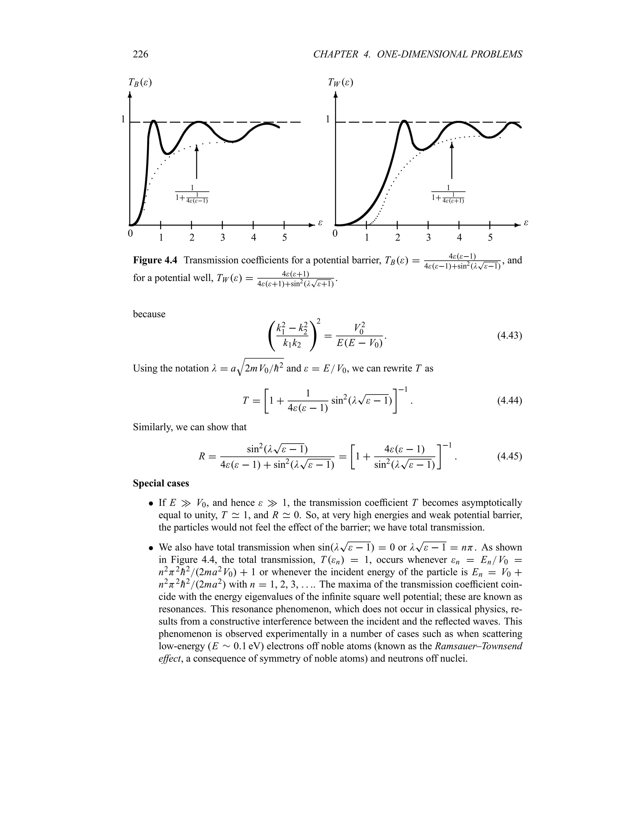
![230 CHAPTER 4. ONE-DIMENSIONAL PROBLEMS
-
6
x1 x2
E
x
Vx
(a)
-
6
x
Vx
E
x1 x2
xi
(b)
Figure 4.5 (a) Tunneling though a potential barrier. (b) Approximation of a smoothly varying
potential Vx by square barriers.
would be negative; the points x x1 and x x2 are known as the classical turning points.
Quantum mechanically, however, since particles display wave features, the quantum waves can
tunnel through the barrier.
As shown in the square barrier example, the particle has a finite probability of tunneling
through the barrier. In this case we managed to find an analytical expression (4.67) for the tun-
neling probability only because we dealt with a simple square potential. Analytic expressions
cannot be obtained for potentials with arbitrary spatial dependence. In such cases one needs
approximations. The Wentzel–Kramers–Brillouin (WKB) method (Chapter 9) provides one of
the most useful approximation methods. We will show that the transmission coefficient for a
barrier potential Vx is given by
T r exp
|
2
h
= x2
x1
dx
S
2m [Vx E]
}
(4.69)
We can obtain this relation by means of a crude approximation. For this, we need simply to take
the classically forbidden region x1 x x2 (Figure 4.5b) and divide it into a series of small
intervals xi . If xi is small enough, we may approximate the potential Vxi at each point xi
by a square potential barrier. Thus, we can use (4.68) to calculate the transmission probability
corresponding to Vxi :
Ti r exp
v
2xi
h
S
2mVxi E
w
(4.70)
The transmission probability for the general potential of Figure 4.5, where we divided the region
x1 x x2 into a very large number of small intervals xi , is given by
T r lim
N*
N
i1
exp
v
2xi
h
S
2mVxi E
w
exp
2
h
lim
xi 0
;
i
xi
S
2mVxi E
exp
v
2
h
= x2
x1
dx
S
2m [Vx E]
w
(4.71)](https://image.slidesharecdn.com/zettili-250217213640-909f6141/75/Zettili-Quantum-mechanics-Concept-and-application-pdf-247-2048.jpg)


![234 CHAPTER 4. ONE-DIMENSIONAL PROBLEMS
This energy is too small to be detected, much less measured, by any known experimental tech-
nique.
(b) For the zero-point energy of an oxygen atom confined to a 2 1010 m lattice, since
the oxygen atom has 16 nucleons, its mass is of the order of m 16 16 1027 kg
26 1027 kg, so we have
E
1067 J
2 26 1027 4 1020
05 1022
J 3 104
eV (4.85)
(c) The zero-point energy of an electron m r 1030 kg that is confined to an atom (a r 1
1010 m ) is
E
1067 J
2 1030 1020
5 1018
J 30 eV (4.86)
This energy is important at the atomic scale, for the binding energy of a hydrogen electron is
about 14 eV. So the zero-point energy is negligible for macroscopic objects, but important for
microscopic systems.
4.6.2 The Symmetric Potential Well
What happens if the potential (4.72) is translated to the left by a distance of a2 to become
symmetric?
Vx
* x a2
0 a2 n x n a2
* x a2
(4.87)
First, we would expect the energy spectrum (4.76) to remain unaffected by this translation,
since the Hamiltonian is invariant under spatial translations; as it contains only a kinetic part,
it commutes with the particle’s momentum, [H P] 0. The energy spectrum is discrete and
nondegenerate.
Second, earlier in this chapter we saw that for symmetric potentials, Vx Vx, the
wave function of bound states must be either even or odd. The wave function corresponding to
the potential (4.87) can be written as follows:
Onx
U
2
a
sin
KnH
a
r
x
a
2
sL
T
2
a cosnH
a x n 1 3 5 7
T
2
a sinnH
a x n 2 4 6 8
(4.88)
That is, the wave functions corresponding to odd quantum numbers n 1 3 5 are sym-
metric, Ox Ox, and those corresponding to even numbers n 2 4 6 are antisym-
metric, Ox Ox.
4.7 The Finite Square Well Potential
Consider a particle of mass m moving in the following symmetric potential:
Vx
V0 x a2
0 a2 n x n a2
V0 x a2
(4.89)](https://image.slidesharecdn.com/zettili-250217213640-909f6141/75/Zettili-Quantum-mechanics-Concept-and-application-pdf-251-2048.jpg)
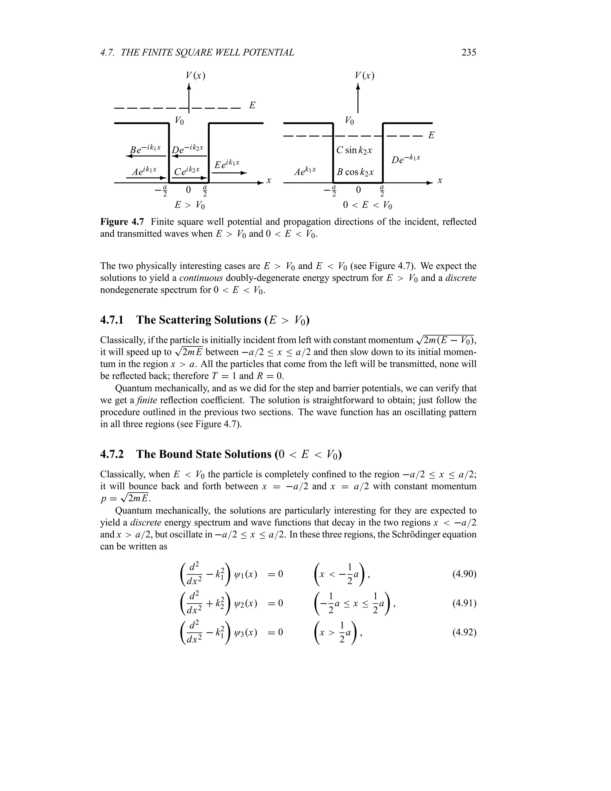
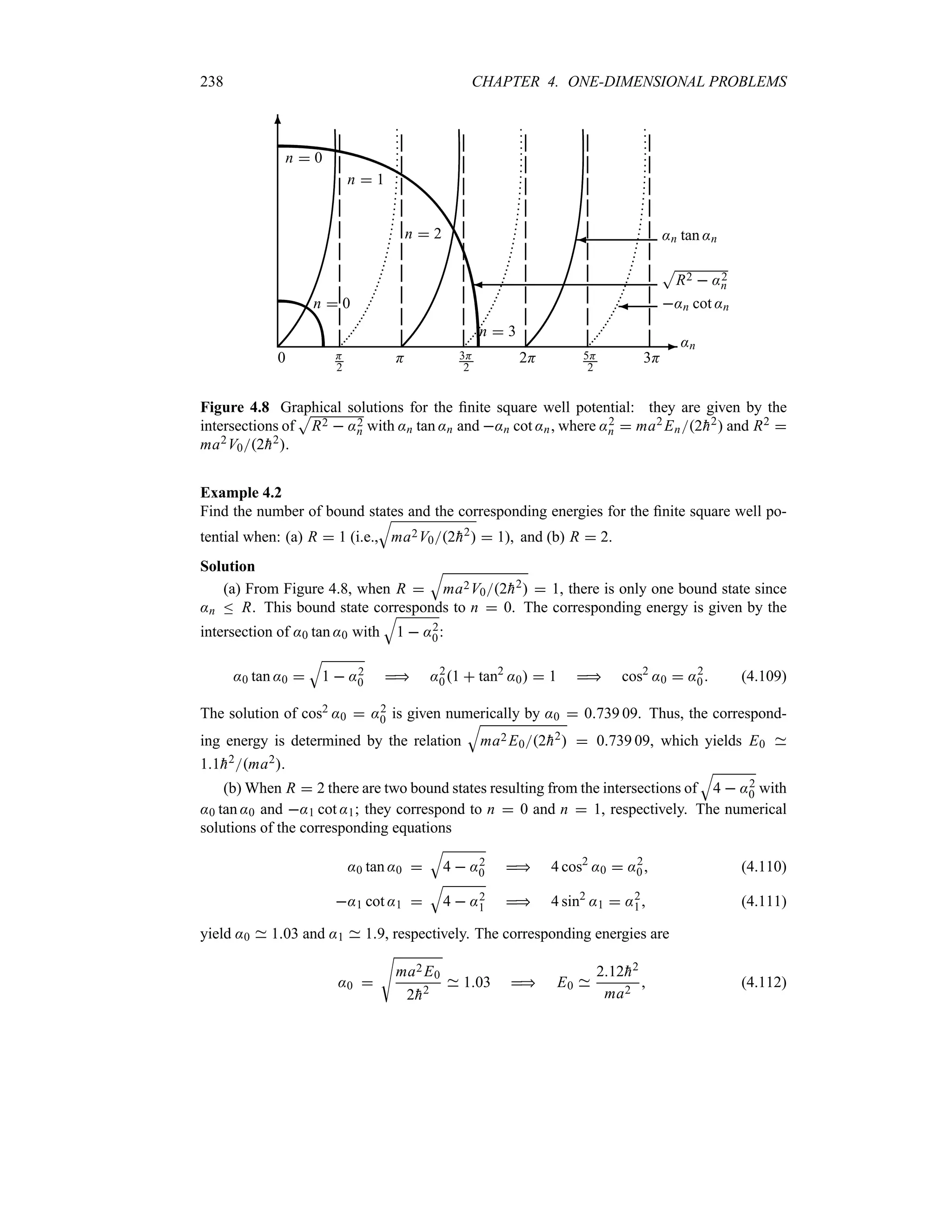
![240 CHAPTER 4. ONE-DIMENSIONAL PROBLEMS
f x expx22x2
0, where f x is a function of x. Inserting this trial function into (4.116),
we obtain a differential equation for f x. This new differential equation can be solved by
expanding f x out in a power series (i.e., f x
3*
n0 anxn, where an is just a coefficient),
which when inserted into the differential equation leads to a recursion relation. By demanding
the power series of f x to terminate at some finite value of n (because the wave function
Ox has to be finite everywhere, notably when x *), the recursion relation yields an
expression for the energy eigenvalues which are discrete or quantized:
En
t
n
1
2
u
h n 0 1 2 3 (4.117)
After some calculations, we can show that the wave functions that are physically acceptable
and that satisfy (4.116) are given by
Onx
1
ST
H2nn!x0
ex22x2
0 Hn
t
x
x0
u
(4.118)
where Hny are nth order polynomials called Hermite polynomials:
Hny 1n
ey2 dn
dyn
ey2
(4.119)
From this relation it is easy to calculate the first few polynomials:
H0y 1 H1y 2y
H2y 4y2 2 H3y 8y3
12y (4.120)
H4y 16y4 48y2 12 H5y 32y5
160y3
120y
We will deal with the physical interpretations of the harmonic oscillator results when we study
the second method.
Algebraic method
Let us now show how to solve the harmonic oscillator eigenvalue problem using the algebraic
method. For this, we need to rewrite the Hamiltonian (4.114) in terms of the two Hermitian,
dimensionless operators p P
T
m
h and q X
T
m
h:
H
h
2
p2
q2
(4.121)
and then introduce two non-Hermitian, dimensionless operators:
a
1
T
2
q i p a†
1
T
2
q i p (4.122)
The physical meaning of the operators a and a† will be examined later. Note that
a†a
1
2
q i pq i p
1
2
q2
p2
iq p i pq
1
2
q2
p2
i
2
[q p] (4.123)
where, using [X P] i
h, we can verify that the commutator between q and p is
d
q p
e
vU
m
h
X
1
T
hm
P
w
1
h
K
X P
L
i (4.124)](https://image.slidesharecdn.com/zettili-250217213640-909f6141/75/Zettili-Quantum-mechanics-Concept-and-application-pdf-257-2048.jpg)
![4.8. THE HARMONIC OSCILLATOR 241
hence
a†a
1
2
q2
p2
1
2
(4.125)
or
1
2
q2
p2
a†a
1
2
(4.126)
Inserting (4.126) into (4.121) we obtain
H
h
t
a†a
1
2
u
h
t
N
1
2
u
with N a†a (4.127)
where N is known as the number operator or occupation number operator, which is clearly
Hermitian.
Let us now derive the commutator [a a†]. Since [X P] i
h we have [q p] 1
h [X P]
i; hence
[a a†]
1
2
d
q i p q i p
e
i
d
q p
e
1 (4.128)
or
[a a†] 1 (4.129)
4.8.1 Energy Eigenvalues
Note that H as given by (4.127) commutes with N, since H is linear in N. Thus, H and N can
have a set of joint eigenstates, to be denoted by nO:
N nO n nO (4.130)
and
H nO En nO (4.131)
the states nO are called energy eigenstates. Combining (4.127) and (4.131), we obtain the
energy eigenvalues at once:
En
t
n
1
2
u
h (4.132)
We will show later that n is a positive integer; it cannot have negative values.
The physical meaning of the operators a, a†, and N can now be clarified. First, we need the
following two commutators that can be extracted from (4.129) and (4.127):
[a H]
ha [a† H]
ha† (4.133)
These commutation relations along with (4.131) lead to
H
b
a nO
c
aH
ha nO En
h
b
a nO
c
(4.134)
H
r
a† nO
s
a†H
ha† nO En
h a† nO (4.135)
Thus, a nO and a† nO are eigenstates of H with eigenvalues En
h and En
h,
respectively. So the actions of a and a† on nO generate new energy states that are lower and](https://image.slidesharecdn.com/zettili-250217213640-909f6141/75/Zettili-Quantum-mechanics-Concept-and-application-pdf-258-2048.jpg)
![242 CHAPTER 4. ONE-DIMENSIONAL PROBLEMS
higher by one unit of
h, respectively. As a result, a and a† are respectively known as the
lowering and raising operators, or the annihilation and creation operators; they are also known
as the ladder operators.
Let us now find out how the operators a and a† act on the energy eigenstates nO. Since
a and a† do not commute with N, the states nO are eigenstates neither to a nor to a†. Using
(4.129) along with [AB C] A[B C] [A C]B, we can show that
[N a] a [N a†] a† (4.136)
hence Na aN 1 and Na† a†N 1. Combining these relations with (4.130), we
obtain
N
b
a nO
c
aN 1 nO n 1
b
a nO
c
(4.137)
N
r
a† nO
s
a†N 1 nO n 1a† nO (4.138)
These relations reveal that a nO and a† nO are eigenstates of N with eigenvalues n 1
and n 1, respectively. This implies that when a and a† operate on nO, respectively, they
decrease and increase n by one unit. That is, while the action of a on nO generates a new state
n 1O (i.e., a nO r n 1O), the action of a† on nO generates n 1O. Hence from (4.137)
we can write
a nO cn n 1O (4.139)
where cn is a constant to be determined from the requirement that the states nO be normalized
for all values of n. On the one hand, (4.139) yields
r
Nn a†
s
b
a nO
c
Nn a†a nO cn
2
Nn 1 n 1O cn
2
(4.140)
and, on the other hand, (4.130) gives
r
Nn a†
s
b
a nO
c
Nn a†a nO nNn nO n (4.141)
When combined, the last two equations yield
cn
2
n (4.142)
This implies that n, which is equal to the norm of a nO (see (4.141)), cannot be negative,
n o 0, since the norm is a positive quantity. Substituting (4.142) into (4.139) we end up with
a nO
T
n n 1O (4.143)
This equation shows that repeated applications of the operator a on nO generate a sequence of
eigenvectors n 1O n 2O n 3O . Since n o 0 and since a 0O 0, this sequence
has to terminate at n 0; this is true if we start with an integer value of n. But if we start with
a noninteger n, the sequence will not terminate; hence it leads to eigenvectors with negative
values of n. But as shown above, since n cannot be negative, we conclude that n has to be a
nonnegative integer.](https://image.slidesharecdn.com/zettili-250217213640-909f6141/75/Zettili-Quantum-mechanics-Concept-and-application-pdf-259-2048.jpg)
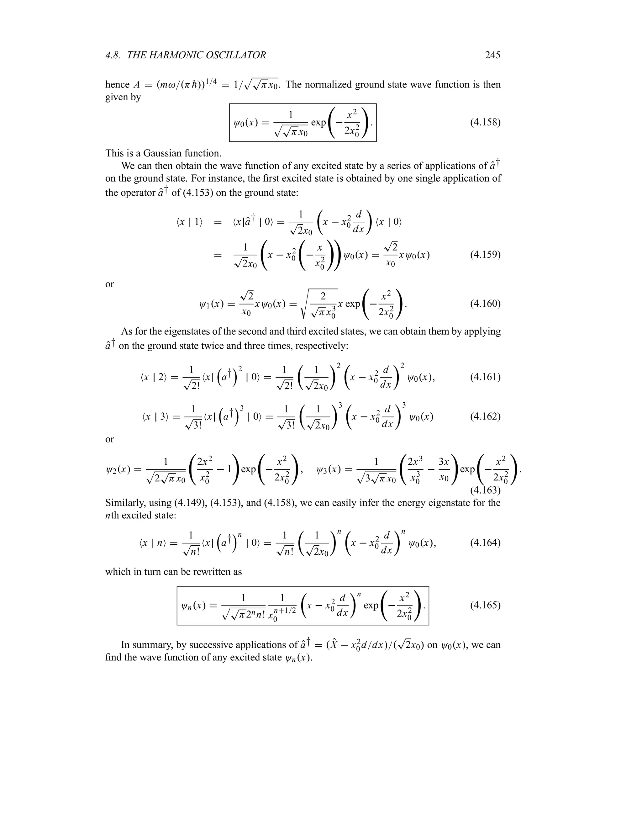
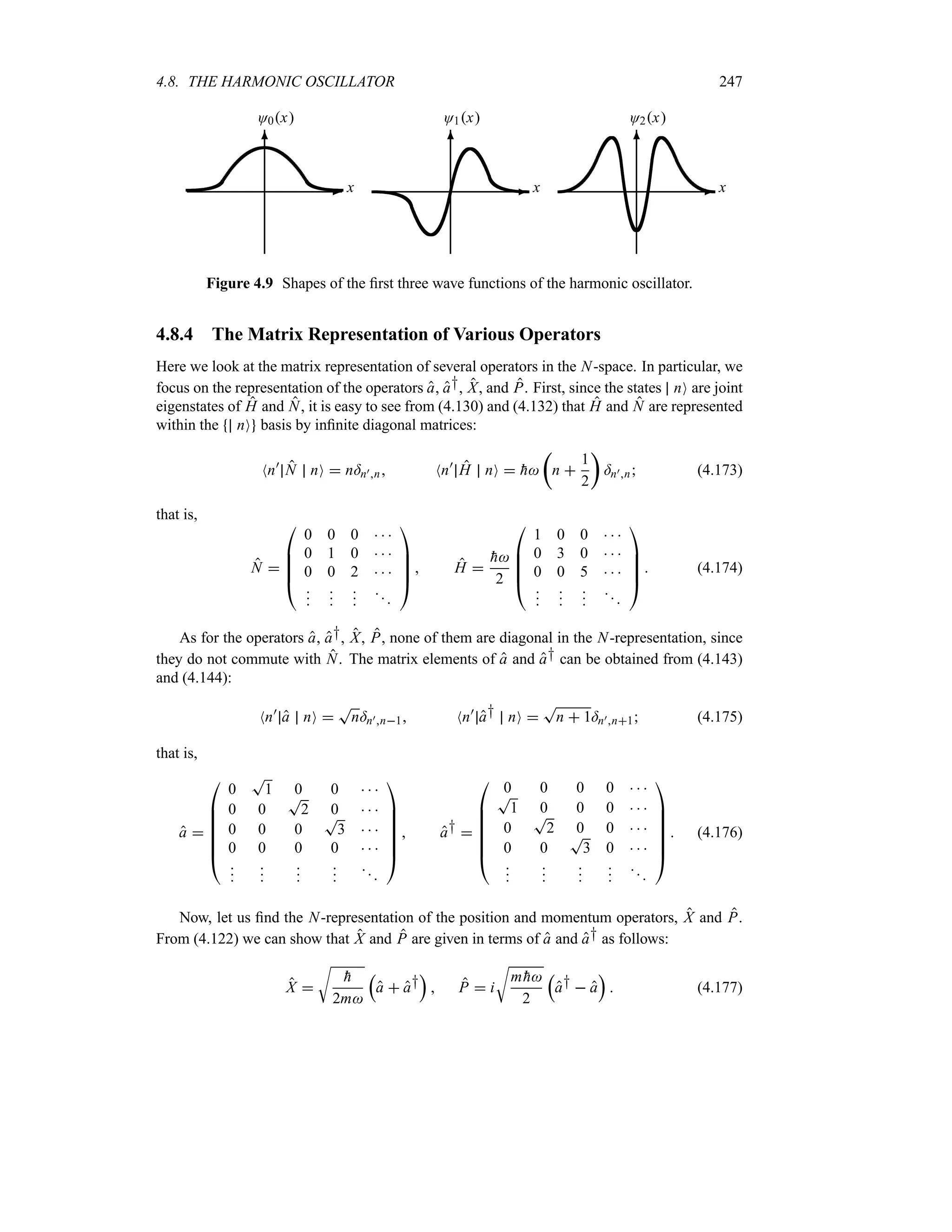
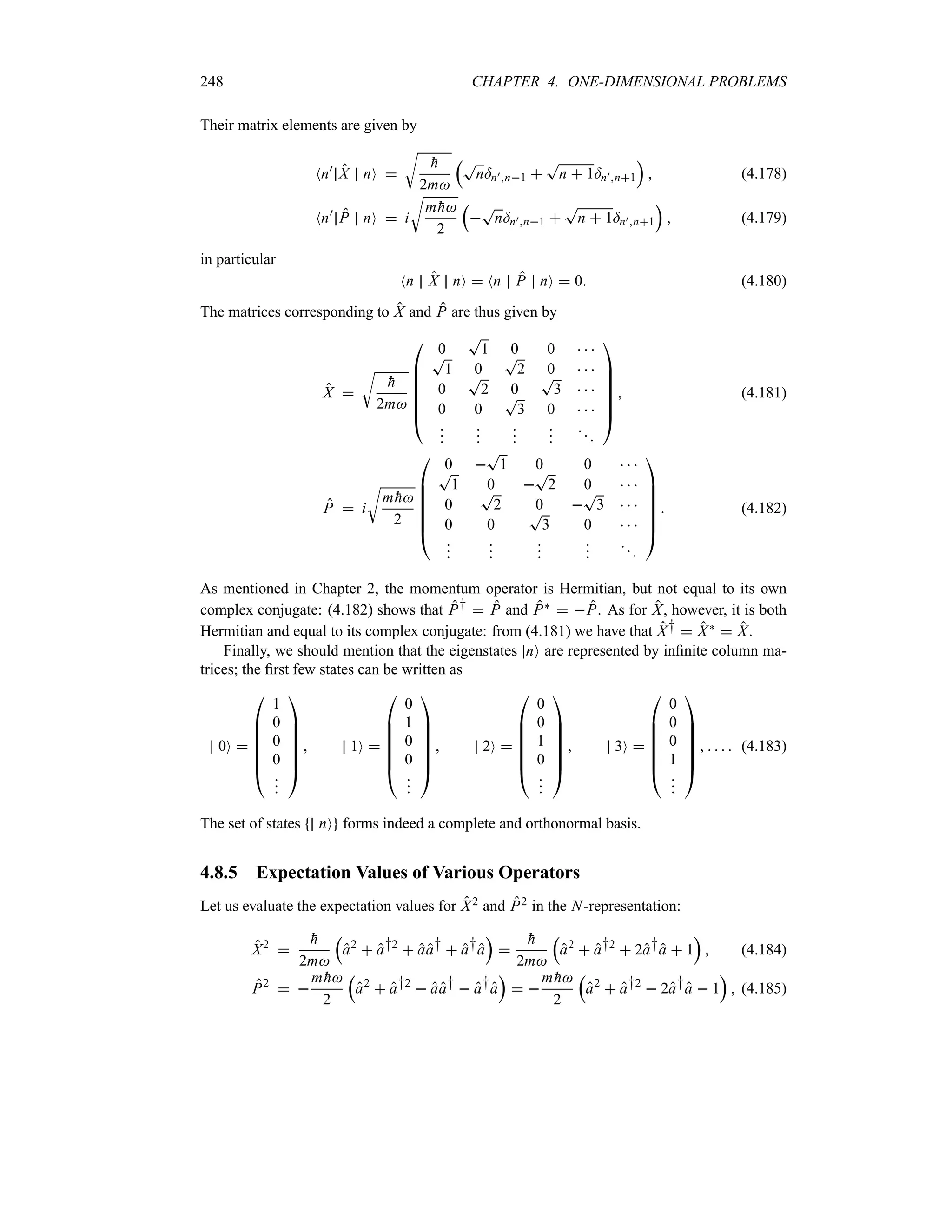
![4.9. NUMERICAL SOLUTION OF THE SCHRÖDINGER EQUATION 249
where we have used the fact that aa† a†a 2a†a 1. Since the expectation values of a2
and a†2 are zero, Nn a2 nO Nn a†2 nO 0, and Nn a†a nO n, we have
Nn aa† a†a nO Nn 2a†a 1 nO 2n 1 (4.186)
hence
Nn X2
nO
h
2m
Nn aa† a†a nO
h
2m
2n 1 (4.187)
Nn P2
nO
m
h
2
Nn aa† a†a nO
m
h
2
2n 1 (4.188)
Comparing (4.187) and (4.188) we see that the expectation values of the potential and kinetic
energies are equal and are also equal to half the total energy:
m2
2
Nn X2
nO
1
2m
Nn P2
nO
1
2
Nn H nO (4.189)
This result is known as the Virial theorem.
We can now easily calculate the product xp from (4.187) and (4.188). Since NXO
NPO 0 we have
x
T
NX2O NXO2
T
NX2O
U
h
2m
2n 1 (4.190)
p
T
NP2O NPO2
T
NP2O
U
m
h
2
2n 1 (4.191)
hence
xp
t
n
1
2
u
h xp o
h
2
(4.192)
since n o 0; this is the Heisenberg uncertainty principle.
4.9 Numerical Solution of the Schrödinger Equation
In this section we are going to show how to solve a one-dimensional Schrödinger equation
numerically. The numerical solutions provide an idea about the properties of stationary states.
4.9.1 Numerical Procedure
We want to solve the following equation numerically:
h2
2m
d2O
dx2
VxOx EOx
d2O
dx2
k2
Ox 0 (4.193)
where k2 2m[E Vx]
h2.
First, divide the x-axis into a set of equidistant points with a spacing of h0 x, as shown
in Figure 4.10a. The wave function Ox can be approximately described by its values at the](https://image.slidesharecdn.com/zettili-250217213640-909f6141/75/Zettili-Quantum-mechanics-Concept-and-application-pdf-266-2048.jpg)
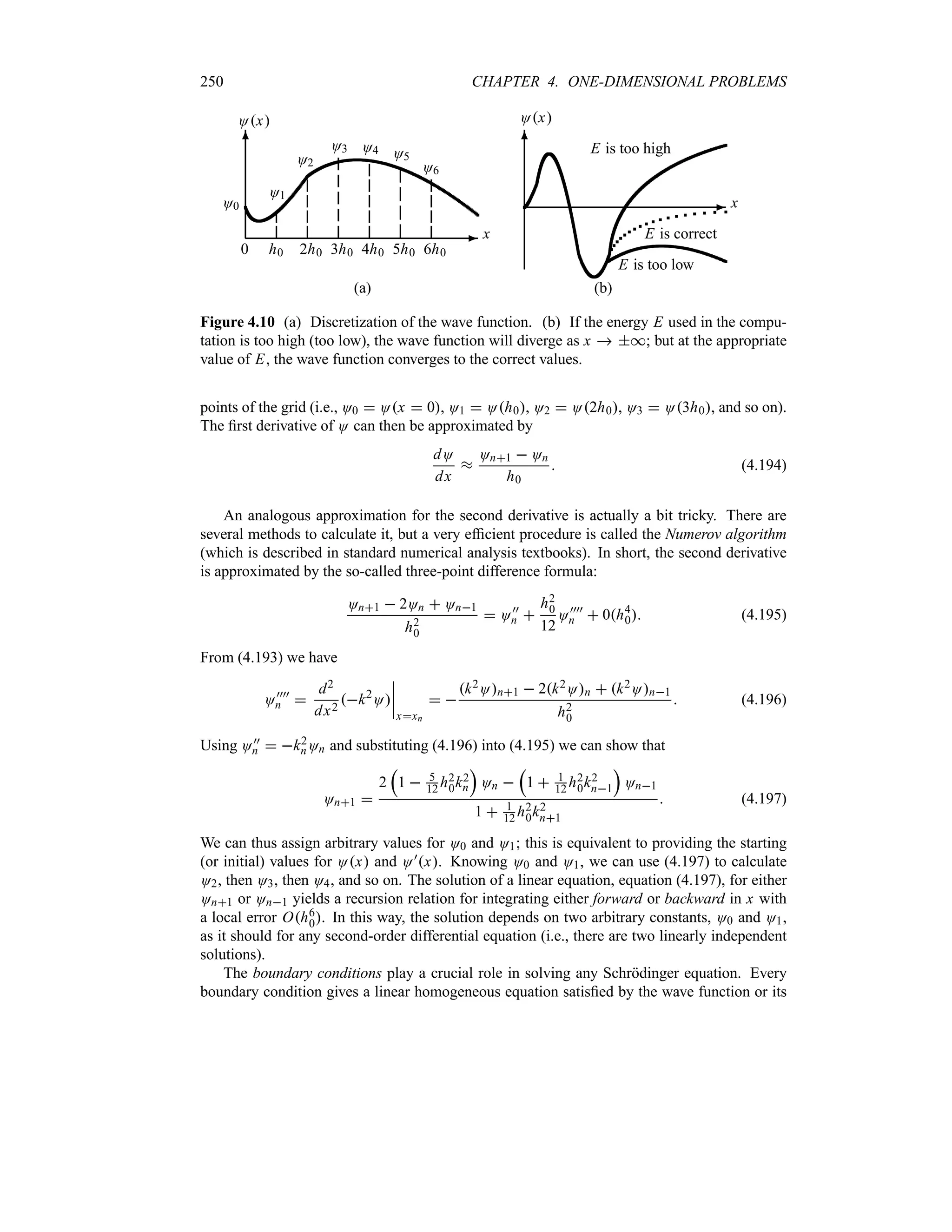

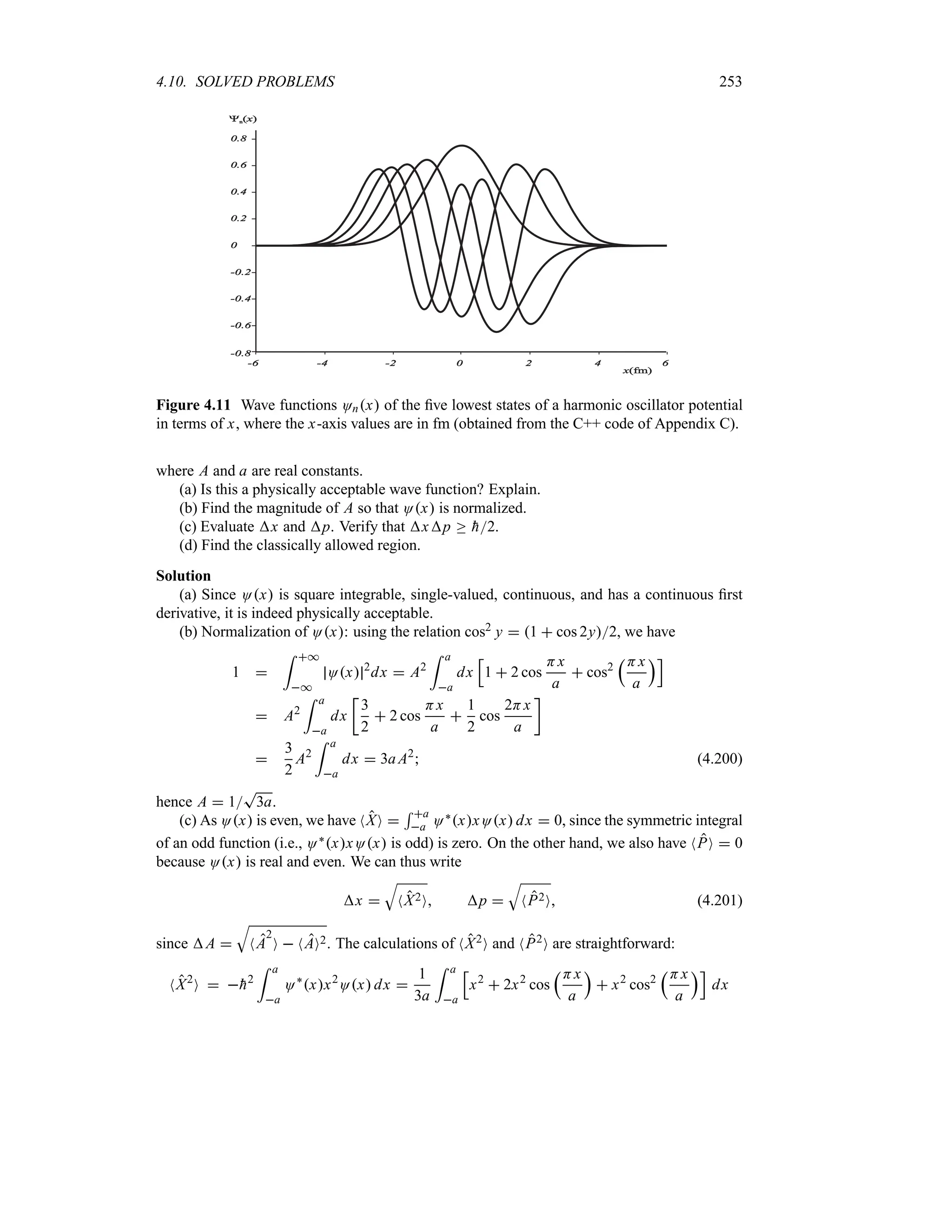

![4.10. SOLVED PROBLEMS 259
(d) The case E 0 corresponds to a free motion and the energy levels represent a contin-
uum. The solution of the Schrödinger equation for E 0 is given by
Ox
|
Ox Aeikx Beikx x 0
Ox Ceikx x 0
(4.236)
where k
T
2mE
h; this corresponds to a plane wave incident from the left together with a
reflected wave in the region x 0, and only a transmitted wave for x 0.
The values of the constants A and B are to be found from the continuity relations. On the
one hand, the continuity of Ox at x 0 yields
A B C (4.237)
and, on the other hand, substituting (4.236) into (4.228), we end up with
ikC A B
2mV0
h2
C 0 (4.238)
Solving (4.237) and (4.238) for BA and CA, we find
B
A
1
1 ik
h2
mV0
C
A
1
1 imV0
h2k
(4.239)
Thus, the reflection and transmission coefficients are
R
n
n
n
n
B
A
n
n
n
n
2
1
1
h4k2
m2V 2
0
1
1 2
h2 E
mV2
0
T
n
n
n
n
C
A
n
n
n
n
2
1
1
m2V2
0
h4k2
1
1
mV2
0
2
h2 E
(4.240)
with R T 1.
Problem 4.5
A particle of mass m is subject to an attractive double-delta potential Vx V0=x a
V0=x a, where V0 0. Consider only the case of negative energies.
(a) Obtain the wave functions of the bound states.
(b) Derive the eigenvalue equations.
(c) Specify the number of bound states and the limit on their energies. Is the ground state
an even state or an odd state?
(d) Estimate the ground state energy for the limits a 0 and a *.
Solution
(a) The Schrödinger equation for this problem is
d2Ox
dx2
2mV0
h2
[=x a =x a] Ox
2mE
h2
Ox 0 (4.241)
For x / a this equation becomes
d2Ox
dx2
2mE
h2
Ox 0 or
d2Ox
dx2
k2
Ox 0 (4.242)](https://image.slidesharecdn.com/zettili-250217213640-909f6141/75/Zettili-Quantum-mechanics-Concept-and-application-pdf-276-2048.jpg)
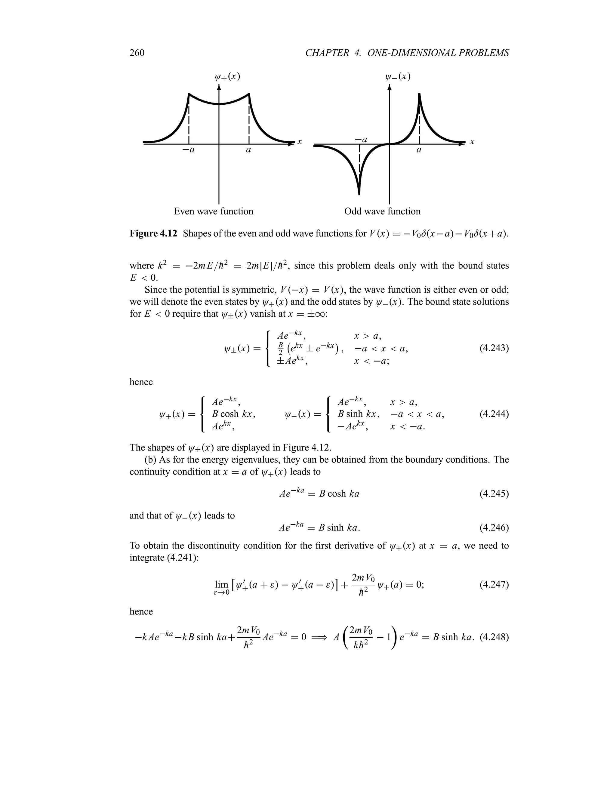
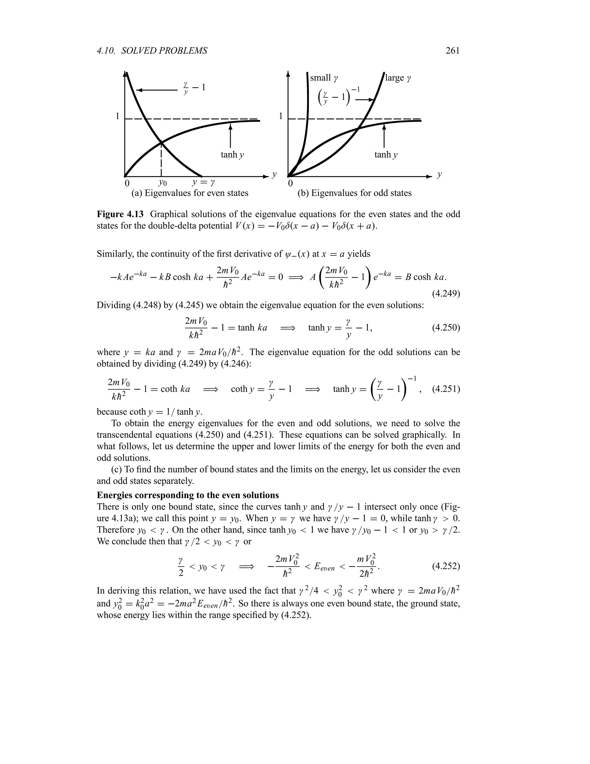
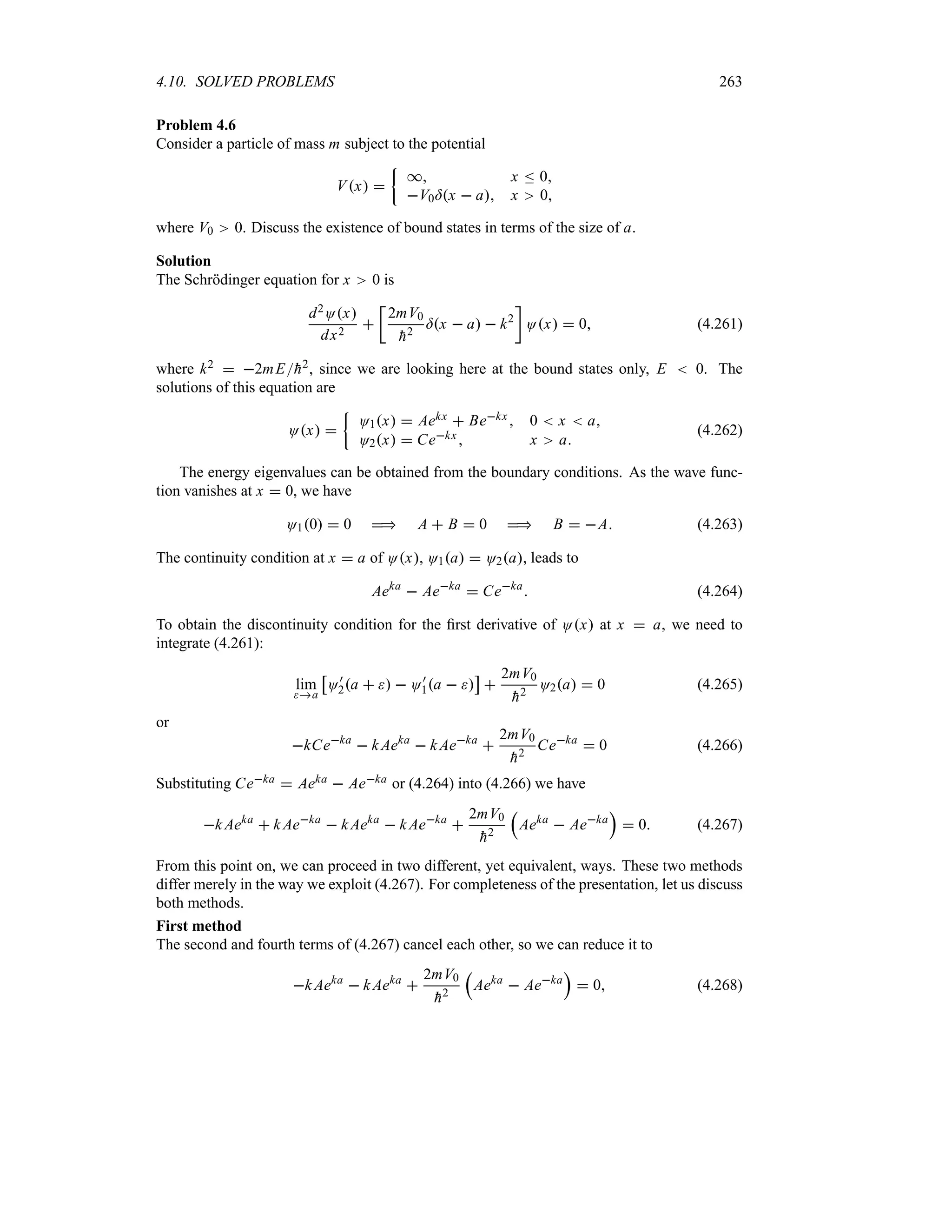
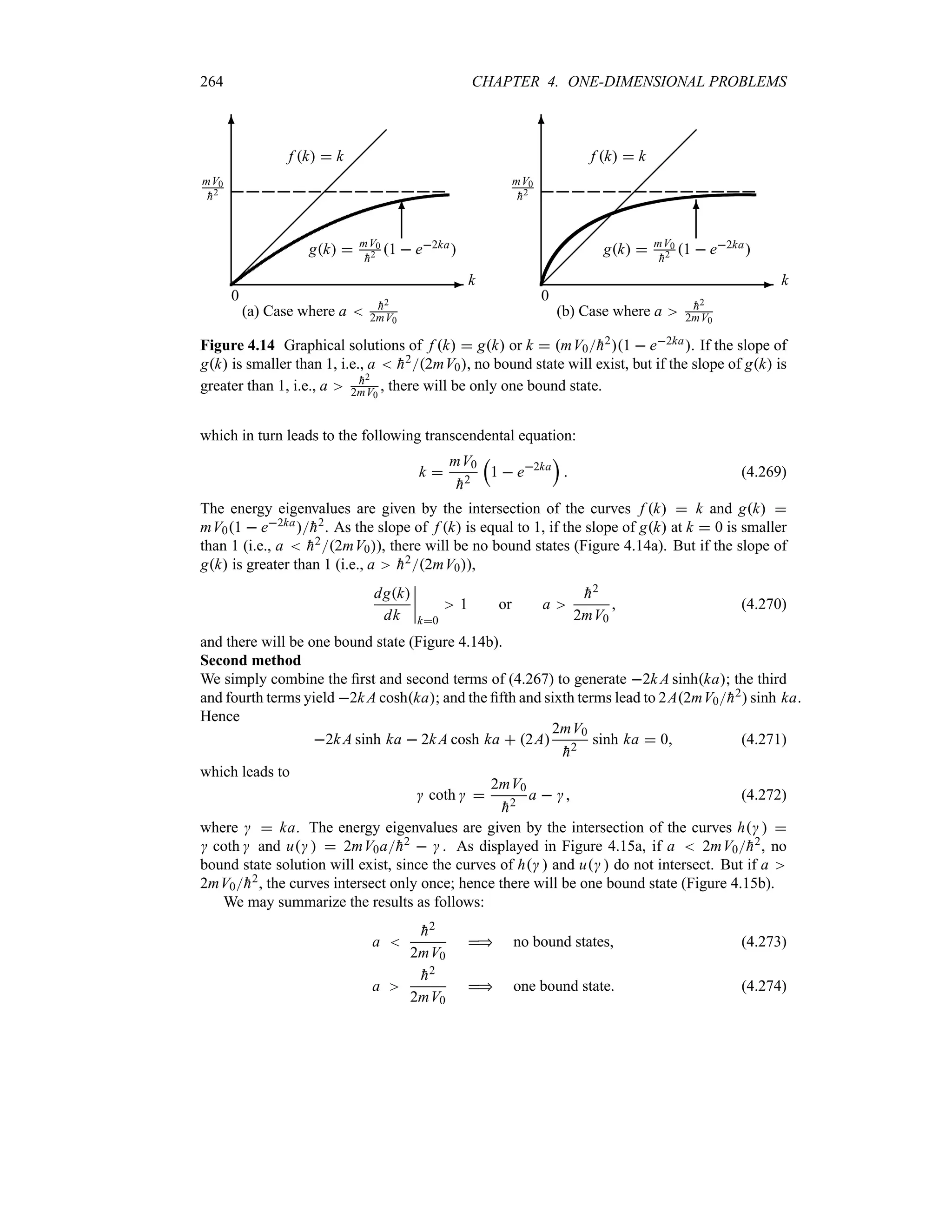


![268 CHAPTER 4. ONE-DIMENSIONAL PROBLEMS
The energy levels of the sphere are practically indistinguishable; the spacings between
the levels are negligible. The energy spectrum therefore forms a continuum; hence the
quantum effects are not noticeable for the sphere.
(c) According to the uncertainty principle, the speed is proportional to ) r
hma. For the
electron, the typical distances are atomic, a 1010 m; hence
) r
hc
mc2a
c r
200 MeV fm
05 MeV 105 fm
c 4 103
c 12 106
m s1
(4.290)
where c is the speed of light. The electron therefore moves quite fast; this is expected since we
have confined the electron to move within a small region.
For the sphere, the typical distances are in the range of 1 cm:
) r
h
ma
r
66 1034 J s
103 kg 102 m
66 1029
m s1
(4.291)
At this speed the sphere is practically at rest.
Problem 4.11
(a) Verify that the matrices representing the operators X and P in the N-space for a har-
monic oscillator obey the correct commutation relation [X P] i
h.
(b) Show that the energy levels of the harmonic oscillator can be obtained by inserting the
matrices of X and P into the Hamiltonian H P22m 1
2 m2 X2.
Solution
(a) Using the matrices of X and P in (4.181) and (4.182), we obtain
X P i
h
2
%
%
%
#
1 0
T
2
0 1 0
T
2 0 1
$
P X i
h
2
%
%
%
#
1 0
T
2
0 1 0
T
2 0 1
$
(4.292)
hence
X P P X i
h
%
%
%
#
1 0 0
0 1 0
0 0 1
$
(4.293)
or [X P] i
hI, where I is the unit matrix.
(b) Again, using the matrices of X and P in (4.181) and (4.182), we can verify that
X2
h
2m
%
%
%
#
1 0
T
2
0 3 0
T
2 0 5
$
P2
m
h
2
%
%
%
#
1 0
T
2
0 3 0
T
2 0 5
$
(4.294)](https://image.slidesharecdn.com/zettili-250217213640-909f6141/75/Zettili-Quantum-mechanics-Concept-and-application-pdf-285-2048.jpg)


![274 CHAPTER 4. ONE-DIMENSIONAL PROBLEMS
Note that the sets X P and x p are conjugate variables separately: [X P] i
h, [x p]
i
h, [X p] [x P] 0. Taking p1, p2, x1, and x2 of (4.328) and (4.329) and inserting them
into (4.325), we obtain
H
1
2m1
rm1
M
P p
s2
1
2
m12
rm2
M
x X
s2
1
2m2
rm2
M
P p
s2
1
2
m22
r
m1
M
x X
s2
1
2
K x2
HCM Hrel (4.330)
where
HC M
1
2M
P2
1
2
M2
X2
Hrel
1
2E
p2
1
2
EP2
x2
(4.331)
with P2 2 kE. We have thus reduced the Hamiltonian of these two coupled harmonic
oscillators to the sum of two independent harmonic oscillators, one with frequency and mass
M and the other of mass E and frequency P
S
2 kE. That is, by introducing the
CM and relative motion variables, we have managed to eliminate the coupled term from the
Hamiltonian.
The energy levels of this two-oscillator system can be inferred at once from the suggestive
Hamiltonians of (4.331):
En1n2
h
t
n1
1
2
u
hP
t
n2
1
2
u
(4.332)
The states of this two-particle system are given by the product of the two states NO n1O n2O;
hence the total wave function, OnX x, is equal to the product of the center of mass wave func-
tion, On1 X, and the wave function of the relative motion, On2 x: OnX x On1 XOn2 x.
Note that both of these wave functions are harmonic oscillator functions whose forms can be
found in (4.172):
OnX x
1
T
H
S
2n1 2n2 n1!n2!x01 x02
e
X22x2
01 e
x22x2
02 Hn1
t
X
x01
u
Hn2
t
x
x02
u
(4.333)
where n n1 n2, x01
T
hM, and x02
T
hEP.
Problem 4.17
Consider a particle of mass m and charge q moving under the influence of a one-dimensional
harmonic oscillator potential. Assume it is placed in a constant electric field E. The Hamil-
tonian of this particle is therefore given by H P22m 1
2 m2 X2 qE X. Derive the
energy expression and the wave function of the nth excited state.
Solution
To find the eigenenergies of the Hamiltonian
H
1
2m
P2
1
2
m2
X2
qE X (4.334)
it is convenient to use the change of variable y X qEm2. Thus the Hamiltonian
becomes
H
1
2m
P2
1
2
m2
y2
q2E2
2m2
(4.335)](https://image.slidesharecdn.com/zettili-250217213640-909f6141/75/Zettili-Quantum-mechanics-Concept-and-application-pdf-291-2048.jpg)
![4.10. SOLVED PROBLEMS 275
Since the term q2E22m2 is a mere constant and P22m 1
2 m2y2 HH O has the
structure of a harmonic oscillator Hamiltonian, we can easily infer the energy levels:
En Nn H nO
h
t
n
1
2
u
q2E2
2m2
(4.336)
The wave function is given by Ony Onx qEm2, where Ony is given in (4.172):
Ony
1
ST
H2nn!x0
ey22x2
0 Hn
t
y
x0
u
(4.337)
Problem 4.18
Consider a particle of mass m that is bouncing vertically and elastically on a smooth reflecting
floor in the Earth’s gravitational field
Vz
|
mgz z 0
* z n 0
where g is a constant (the acceleration due to gravity). Find the energy levels and wave function
of this particle.
Solution
We need to solve the Schrödinger equation with the boundary conditions O0 0 and
O* 0:
h2
2m
d2Oz
dz2
mgzOz EOz
d2Oz
dz2
2m
h2
mgz E Oz 0 (4.338)
With the change of variable x
h22m2g232m
h2mgz E, we can reduce this equa-
tion to
d2Mx
dx2
xMx 0 (4.339)
This is a standard differential equation; its solution (which vanishes at x *, i.e.,
M* 0) is given by
Mx BAix where Aix
1
H
= *
0
cos
t
1
3
t3
xt
u
dt (4.340)
where Aix is called the Airy function.
When z 0 we have x 2mg2
h213 E. The boundary condition O0 0 yields
M[2mg2
h213E] 0 or Ai[2mg2
h213 E] 0. The Airy function has zeros
only at certain values of Rn: AiRn 0 with n 0 1 2 3 . The roots Rn of the Airy
function can be found in standard tables. For instance, the first few roots are R0 2338,
R1 4088, R2 5521, R3 6787.
The boundary condition O0 0 therefore gives a discrete set of energy levels which can
be expressed in terms of the roots of the Airy function:
Ai
t
2
mg2
h2
u13
E
0
t
2
mg2
h2
u13
En Rn (4.341)](https://image.slidesharecdn.com/zettili-250217213640-909f6141/75/Zettili-Quantum-mechanics-Concept-and-application-pdf-292-2048.jpg)

![4.11. EXERCISES 279
where O0x 1
TT
H
ex22, O1x
T
2
T
H
xex22, and O2x 1
T
2
T
H
b
2x2 1
c
ex22.
(a) Calculate xnpn for n 0 1 where xn
T
NOn X2 OnO NOn X OnO2.
(b) Calculate a†O0x, aO0x, a†O1x, aO1x, and aO2x, where the operators a† and
a are defined by a X ddx
T
2 and a† X ddx
T
2.
Exercise 4.13
Consider a particle of mass m that is moving in a one-dimensional infinite potential well with
walls at x 0 and x a which is initially (i.e., at t 0) in the state
Ox 0
1
T
2
[M1x M3x]
where M1x and M3x are the ground and second excited states, respectively.
(a) What is the state vector Ox t for t 0 in the Schrödinger picture.
(b) Find the expectation values NXO, NPO, NX2O, and NP2O with respect to OO.
(c) Evaluate xp and verify that it satisfies the uncertainty principle.
Exercise 4.14
If the state of a particle moving in a one-dimensional harmonic oscillator is given by
OO
1
T
17
0O
3
T
17
1O
2
T
17
2O
U
3
17
3O
where nO represents the normalized nth energy eigenstate, find the expectation values of the
number operator, N, and of the Hamiltonian operator.
Exercise 4.15
Find the number of bound states and the corresponding energies for the finite square well po-
tential when (a) R 7 (i.e.,
T
ma2V02
h2 7) and (b) R 3H.
Exercise 4.16
A ball of mass m 02 kg bouncing on a table located at z 0 is subject to the potential
Vz
|
V0 z 0
mgz z 0
where V0 3 J and g is the acceleration due to gravity.
(a) Describe the spectrum of possible energies (i.e., continuous, discrete, or nonexistent) as
E increases from large negative values to large positive values.
(b) Estimate the order of magnitude for the lowest energy state.
(c) Describe the general shapes of the wave functions O0z and O1z corresponding to the
lowest two energy states and sketch the corresponding probability densities.
Exercise 4.17
Consider a particle of mass m moving in a one-dimensional harmonic oscillator potential, with
X
T
h2ma a† and P i
T
m
h2a† a.
(a) Calculate the product of the uncertainties in position and momentum for the particle in
the fifth excited state, i.e., XP5.
(b) Compare the result of (a) with the uncertainty product when the particle is in its lowest
energy state. Explain why the two uncertainty products are different.](https://image.slidesharecdn.com/zettili-250217213640-909f6141/75/Zettili-Quantum-mechanics-Concept-and-application-pdf-296-2048.jpg)


![284 CHAPTER 5. ANGULAR MOMENTUM
The Cartesian components of ;
L are
Lx Y Pz Z Py i
h
t
Y
z
Z
y
u
(5.3)
Ly Z Px X Pz i
h
t
Z
x
X
z
u
(5.4)
Lz X Py Y Px i
h
t
X
y
Y
x
u
(5.5)
Clearly, angular momentum does not exist in a one-dimensional space. We should mention that
the components Lx , Ly, Lz, and the square of ;
L,
;
L
2
L2
x L2
y L2
z (5.6)
are all Hermitian.
Commutation relations
Since X, Y, and Z mutually commute and so do Px , Py, and Pz, and since [X Px ] i
h,
[Y Py] i
h, [Z Pz] i
h, we have
[Lx Ly] [Y Pz Z Py Z Px X Pz]
[Y Pz Z Px ] [Y Pz X Pz] [Z Py Z Px ] [Z Py X Pz]
Y[Pz Z]Px X[Z Pz]Py i
hX Py Y Px
i
hLz (5.7)
A similar calculation yields the other two commutation relations; but it is much simpler to infer
them from (5.7) by means of a cyclic permutation of the xyz components, x y z x:
[Lx Ly] i
hLz [Ly Lz] i
hLx [Lz Lx] i
hLy (5.8)
As mentioned in Chapter 3, since Lx , Ly, and Lz do not commute, we cannot measure them
simultaneously to arbitrary accuracy.
Note that the commutation relations (5.8) were derived by expressing the orbital angular
momentum in the position representation, but since these are operator relations, they must
be valid in any representation. In the following section we are going to consider the general
formalism of angular momentum, a formalism that is restricted to no particular representation.
Example 5.1
(a) Calculate the commutators [X Lx ], [X Ly], and [X Lz].
(b) Calculate the commutators: [Px Lx ], [Px Ly], and [Px Lz].
(c) Use the results of (a) and (b) to calculate [X ;
L2] and [Px ;
L2].](https://image.slidesharecdn.com/zettili-250217213640-909f6141/75/Zettili-Quantum-mechanics-Concept-and-application-pdf-301-2048.jpg)
![5.3. GENERAL FORMALISM OF ANGULAR MOMENTUM 285
Solution
(a) The only nonzero commutator which involves X and the various components of Lx , Ly,
Lz is [X Px] i
h. Having stated this result, we can easily evaluate the needed commutators.
First, since Lx Y Pz Z Py involves no Px , the operator X commutes separately with Y, Pz,
Z, and Py; hence
[X Lx ] [X Y Pz Z Py] 0 (5.9)
The evaluation of the other two commutators is straightforward:
[X Ly] [X Z Px X Pz] [X Z Px ] Z[X Px ] i
hZ (5.10)
[X Lz] [X X Py Y Px] [X Y Px ] Y[X Px ] i
hY (5.11)
(b) The only commutator between Px and the components of Lx, Ly, Lz that survives is
again [Px X] i
h. We may thus infer
[Px Lx ] [Px Y Pz Z Py] 0 (5.12)
[Px Ly] [Px Z Px X Pz] [Px X Pz] [Px X]Pz i
hPz (5.13)
[Px Lz] [Px X Py Y Px ] [Px X Py] [Px X]Py i
hPy (5.14)
(c) Using the commutators derived in (a) and (b), we infer
[X ;
L2
] [X L2
x ] [X L2
y] [X L2
z ]
0 Ly[X Ly] [X Ly]Ly Lz[X Lz] [X Lz]Lz
i
hLy Z Z Ly LzY Y Ly (5.15)
[Px ;
L2
] [Px L2
x] [Px L2
y] [Px L2
z ]
0 Ly[Px Ly] [Px Ly]Ly Lz[Px Lz] [Px Lz]Lz
i
hLy Pz Pz Ly Lz Py Py Ly (5.16)
5.3 General Formalism of Angular Momentum
Let us now introduce a more general angular momentum operator ;
J that is defined by its three
components Jx Jy and Jz, which satisfy the following commutation relations:
[Jx Jy] i
hJz [Jy Jz] i
hJx [Jz Jx] i
hJy (5.17)
or equivalently by
;
J ;
J i
h ;
J (5.18)
Since Jx, Jy, and Jz do not mutually commute, they cannot be simultaneously diagonalized;
that is, they do not possess common eigenstates. The square of the angular momentum,
;
J2
J2
x J2
y J2
z (5.19)](https://image.slidesharecdn.com/zettili-250217213640-909f6141/75/Zettili-Quantum-mechanics-Concept-and-application-pdf-302-2048.jpg)
![286 CHAPTER 5. ANGULAR MOMENTUM
is a scalar operator; hence it commutes with Jx Jy and Jz:
[ ;
J2
Jk] 0 (5.20)
where k stands for x y, and z. For instance, in the the case k x we have
[ ;
J2
Jx] [J2
x Jx ] Jy[Jy Jx ] [Jy Jx]Jy Jz[Jz Jx] [Jz Jx ]Jz
Jyi
hJz i
hJzJy Jzi
hJy i
hJyJz
0 (5.21)
because [J2
x Jx] 0, [Jy Jx] i
hJz, and [Jz Jx ] i
hJy. We should note that the
operators Jx, Jy, Jz, and ;
J2 are all Hermitian; their eigenvalues are real.
Eigenstates and eigenvalues of the angular momentum operator
Since ;
J2 commutes with Jx , Jy and Jz, each component of ;
J can be separately diagonalized
(hence it has simultaneous eigenfunctions) with ;
J2. But since the components Jx , Jy and Jz
do not mutually commute, we can choose only one of them to be simultaneously diagonalized
with ;
J2. By convention we choose Jz. There is nothing special about the z-direction; we can
just as well take ;
J2 and Jx or ;
J2 and Jy.
Let us now look for the joint eigenstates of ;
J2 and Jz and their corresponding eigenvalues.
Denoting the joint eigenstates by : ;O and the eigenvalues of ;
J2 and Jz by
h2: and
h;,
respectively, we have
;
J2
: ;O
h2
: : ;O (5.22)
Jz : ;O
h; : ;O (5.23)
The factor
h is introduced so that : and ; are dimensionless; recall that the angular momentum
has the dimensions of
h and that the physical dimensions of
h are: [
h] energy time. For
simplicity, we will assume that these eigenstates are orthonormal:
N:)
;)
: ;O =:) :=;) ; (5.24)
Now we need to introduce raising and lowering operators J and J, just as we did when
we studied the harmonic oscillator in Chapter 4:
J Jx i Jy (5.25)
This leads to
Jx
1
2
J J Jy
1
2i
J J (5.26)
hence
J2
x
1
4
J2
J J J J J2
J2
y
1
4
J2
J J J J J2
(5.27)
Using (5.17) we can easily obtain the following commutation relations:
[ ;
J2
J] 0 [J J] 2
hJz [Jz J]
hJ (5.28)](https://image.slidesharecdn.com/zettili-250217213640-909f6141/75/Zettili-Quantum-mechanics-Concept-and-application-pdf-303-2048.jpg)
![5.3. GENERAL FORMALISM OF ANGULAR MOMENTUM 287
In addition, J and J satisfy
J J J2
x J2
y
hJz ;
J2
J2
z
hJz (5.29)
J J J2
x J2
y
hJz ;
J2
J2
z
hJz (5.30)
These relations lead to
;
J2
J Jb J2
z b
hJz (5.31)
which in turn yield
;
J2
1
2
J J J J J2
z (5.32)
Let us see how J operate on : ;O. First, since J do not commute with Jz, the kets
: ;O are not eigenstates of J. Using the relations (5.28) we have
JzJ : ;O J Jz
hJ : ;O
h; 1J : ;O (5.33)
hence the ket (J : ;O) is an eigenstate of Jz with eigenvalues
h; 1. Now since Jz and
;
J2 commute, (J : ;O) must also be an eigenstate of ;
J2. The eigenvalue of ;
J2 when acting
on J : ;O can be determined by making use of the commutator [ ;
J2 J] 0. The state
(J : ;O is also an eigenstate of ;
J2 with eigenvalue
h2::
;
J2
J : ;O J ;
J2
: ;O
h2
:J : ;O (5.34)
From (5.33) and (5.34) we infer that when J acts on : ;O, it does not affect the first quantum
number :, but it raises or lowers the second quantum number ; by one unit. That is, J : ;O
is proportional to : ; 1O:
J : ;O C
:; : ; 1O (5.35)
We will determine the constant C
:; later on.
Note that, for a given eigenvalue : of ;
J2, there exists an upper limit for the quantum number
;. This is due to the fact that the operator ;
J2 J2
z is positive, since the matrix elements of
;
J2 J2
z J2
x J2
y are o 0; we can therefore write
N: ; ;
J2
J2
z : ;O
h2
: ;2
o 0 : o ;2
(5.36)
Since ; has an upper limit ;max, there must exist a state : ;maxO which cannot be raised
further:
J : ;max O 0 (5.37)
Using this relation along with J J ;
J2 J2
z
hJz, we see that J J : ;maxO 0 or
;
J2
J2
z
hJz : ;maxO
h2
: ;2
max ;max : ;max O (5.38)](https://image.slidesharecdn.com/zettili-250217213640-909f6141/75/Zettili-Quantum-mechanics-Concept-and-application-pdf-304-2048.jpg)
![290 CHAPTER 5. ANGULAR MOMENTUM
Example 5.2
Calculate [J2
x Jy], [J2
z Jy], and [ ;
J2 Jy]; then show N j m J2
x j mO N j m J2
y
j mO.
Solution
Since [Jx Jy] i
hJz and [Jz Jx ] i
hJy, we have
[J2
x Jy] Jx [Jx Jy] [Jx Jy]Jx i
hJx Jz Jz Jx i
h2Jx Jz i
hJy (5.61)
Similarly, since [Jz Jy] i
hJx and [Jz Jx] i
hJy, we have
[J2
z Jy] Jz[Jz Jy] [Jz Jy]Jz i
hJz Jx Jx Jz i
h2Jx Jz i
hJy (5.62)
The previous two expressions yield
[ ;
J2
Jy] [J2
x J2
y J2
z Jy] [J2
x Jy] [J2
z Jy]
i
h2Jx Jz i
hJy i
h2Jx Jz i
hJy 0 (5.63)
Since we have
J2
x
1
4
J2
J J J J J2
J2
y
1
4
J2
J J J J J2
(5.64)
and since N j m J2
j mO N j m J2
j mO 0, we can write
N j m J2
x j mO
1
4
N j m J J J J j mO N j m J2
y j mO (5.65)
5.4 Matrix Representation of Angular Momentum
The formalism of the previous section is general and independent of any particular representa-
tion. There are many ways to represent the angular momentum operators and their eigenstates.
In this section we are going to discuss the matrix representation of angular momentum where
eigenkets and operators will be represented by column vectors and square matrices, respec-
tively. This is achieved by expanding states and operators in a discrete basis. We will see later
how to represent the orbital angular momentum in the position representation.
Since ;
J2 and Jz commute, the set of their common eigenstates j mO can be chosen as a
basis; this basis is discrete, orthonormal, and complete. For a given value of j, the orthonormal-
ization condition for this base is given by (5.49), and the completeness condition is expressed
by
j
;
m j
j mON j m I (5.66)
where I is the unit matrix. The operators ;
J2 and Jz are diagonal in the basis given by their joint
eigenstates
N j)
m) ;
J2
j mO
h2
j j 1=j) j =m) m (5.67)
N j)
m)
Jz j mO
hm=j) j =m) m (5.68)](https://image.slidesharecdn.com/zettili-250217213640-909f6141/75/Zettili-Quantum-mechanics-Concept-and-application-pdf-307-2048.jpg)
![5.4. MATRIX REPRESENTATION OF ANGULAR MOMENTUM 291
Thus, the matrices representing ;
J2 and Jz in the j mO eigenbasis are diagonal, their diago-
nal elements being equal to
h2 j j 1 and
hm, respectively.
Now since the operators J do not commute with Jz, they are represented in the j mO
basis by matrices that are not diagonal:
N j)
m)
J j mO
h
S
j j 1 mm 1 =j) j =m) m1 (5.69)
We can infer the matrices of Jx and Jy from (5.57) and (5.58):
N j)
m)
Jx j mO
h
2
KS
j j 1 mm 1=m) m1
S
j j 1 mm 1=m) m1
L
=j) j (5.70)
N j)
m)
Jy j mO
h
2i
KS
j j 1 mm 1=m) m1
S
j j 1 mm 1=m) m1
L
=j) j (5.71)
Example 5.3 (Angular momentum j 1)
Consider the case where j 1.
(a) Find the matrices representing the operators ;
J2, Jz, J, Jx , and Jy.
(b) Find the joint eigenstates of ;
J2 and Jz and verify that they form an orthonormal and
complete basis.
(c) Use the matrices of Jx, Jy and Jz to calculate [Jx Jy], [Jy Jz], and [Jz Jx].
(d) Verify that J3
z
h2 Jz and J3
0.
Solution
(a) For j 1 the allowed values of m are 1, 0, 1. The joint eigenstates of ;
J2 and Jz are
1 1O, 1 0O, and 1 1O. The matrix representations of the operators ;
J2 and Jz can be
inferred from (5.67) and (5.68):
;
J2
%
%
#
N1 1 ;
J2 1 1O N1 1 ;
J2 1 0O N1 1 ;
J2 1 1O
N1 0 ;
J2 1 1O N1 0 ;
J2 1 0O N1 0 ;
J2 1 1O
N1 1 ;
J2 1 1O N1 1 ;
J2 1 0O N1 1 ;
J2 1 1O
$
2
h2
#
1 0 0
0 1 0
0 0 1
$ (5.72)
Jz
h
#
1 0 0
0 0 0
0 0 1
$ (5.73)
Similarly, using (5.69), we can ascertain that the matrices of J and J are given by
J
h
T
2
#
0 0 0
1 0 0
0 1 0
$ J
h
T
2
#
0 1 0
0 0 1
0 0 0
$ (5.74)](https://image.slidesharecdn.com/zettili-250217213640-909f6141/75/Zettili-Quantum-mechanics-Concept-and-application-pdf-308-2048.jpg)
![292 CHAPTER 5. ANGULAR MOMENTUM
The matrices for Jx and Jy in the j mO basis result immediately from the relations Jx
J J2 and Jy iJ J2:
Jx
h
T
2
#
0 1 0
1 0 1
0 1 0
$ Jy
h
T
2
#
0 i 0
i 0 i
0 i 0
$ (5.75)
(b) The joint eigenvectors of ;
J2 and Jz can be obtained as follows. The matrix equation of
Jz j mO m
h j mO is
h
#
1 0 0
0 0 0
0 0 1
$
#
a
b
c
$ m
h
#
a
b
c
$
ha m
ha
0 m
hb
hc m
hc
(5.76)
The normalized solutions to these equations for m 1, 0, 1 are respectively given by a 1,
b c 0; a 0, b 1, c 0; and a b 0, c 1; that is,
1 1O
#
1
0
0
$ 1 0O
#
0
1
0
$ 1 1O
#
0
0
1
$ (5.77)
We can verify that these vectors are orthonormal:
N1 m)
1 mO =m) m m)
m 1 0 1 (5.78)
We can also verify that they are complete:
1
;
m1
1 mON1 m
#
0
0
1
$ 0 0 1
#
0
1
0
$ 0 1 0
#
1
0
0
$ 1 0 0
#
1 0 0
0 1 0
0 0 1
$ (5.79)
(c) Using the matrices (5.75) we have
Jx Jy
h2
2
#
0 1 0
1 0 1
0 1 0
$
#
0 i 0
i 0 i
0 i 0
$
h2
2
#
i 0 i
0 0 0
i 0 i
$ (5.80)
Jy Jx
h2
2
#
0 i 0
i 0 i
0 i 0
$
#
0 1 0
1 0 1
0 1 0
$
h2
2
#
i 0 i
0 0 0
i 0 i
$ (5.81)
hence
Jx Jy Jy Jx
h2
2
#
2i 0 0
0 0 0
0 0 2i
$ i
h2
#
1 0 0
0 0 0
0 0 1
$ i
hJz (5.82)
where the matrix of Jz is given by (5.73). A similar calculation leads to [Jy Jz] i
hJx and
[Jz Jx ] i
hJy.](https://image.slidesharecdn.com/zettili-250217213640-909f6141/75/Zettili-Quantum-mechanics-Concept-and-application-pdf-309-2048.jpg)
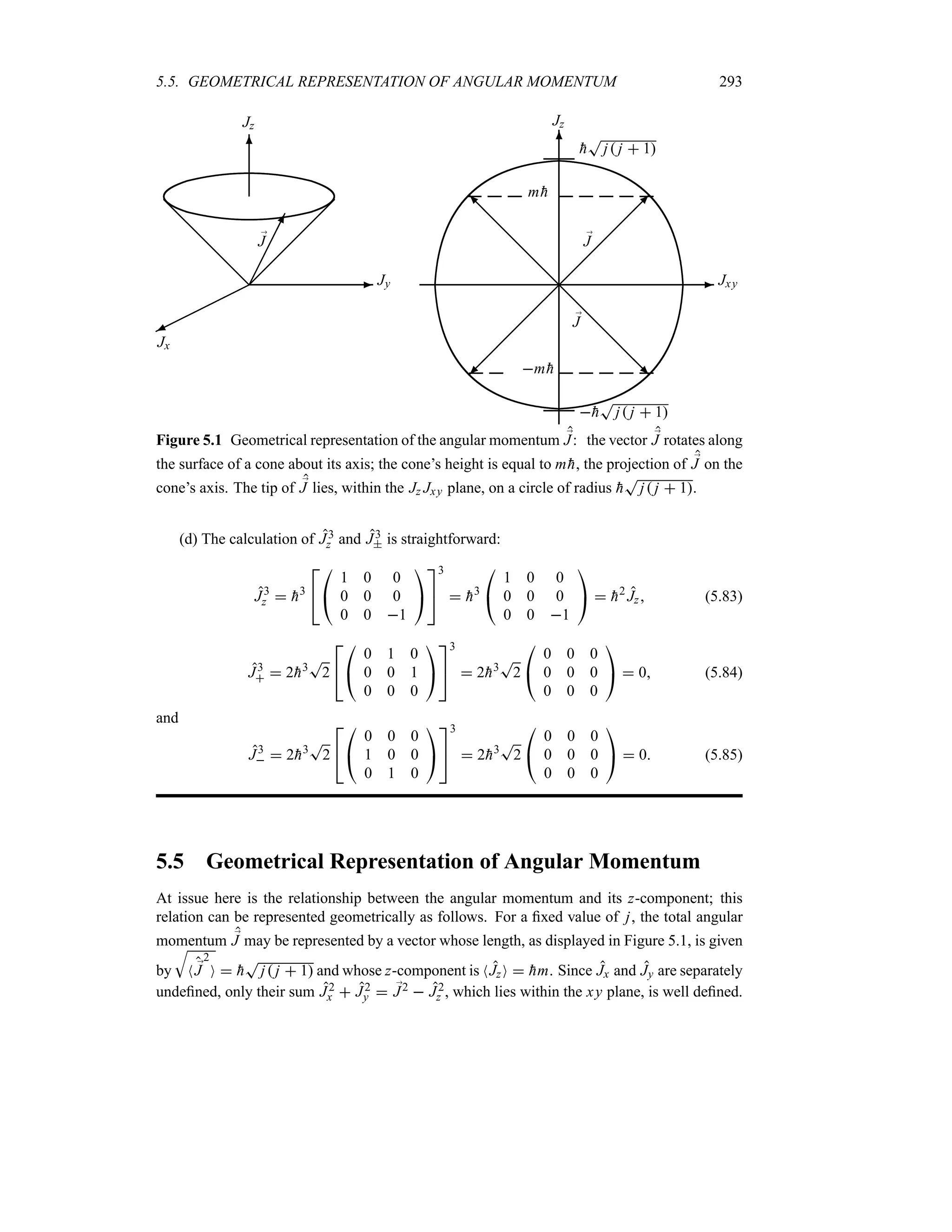
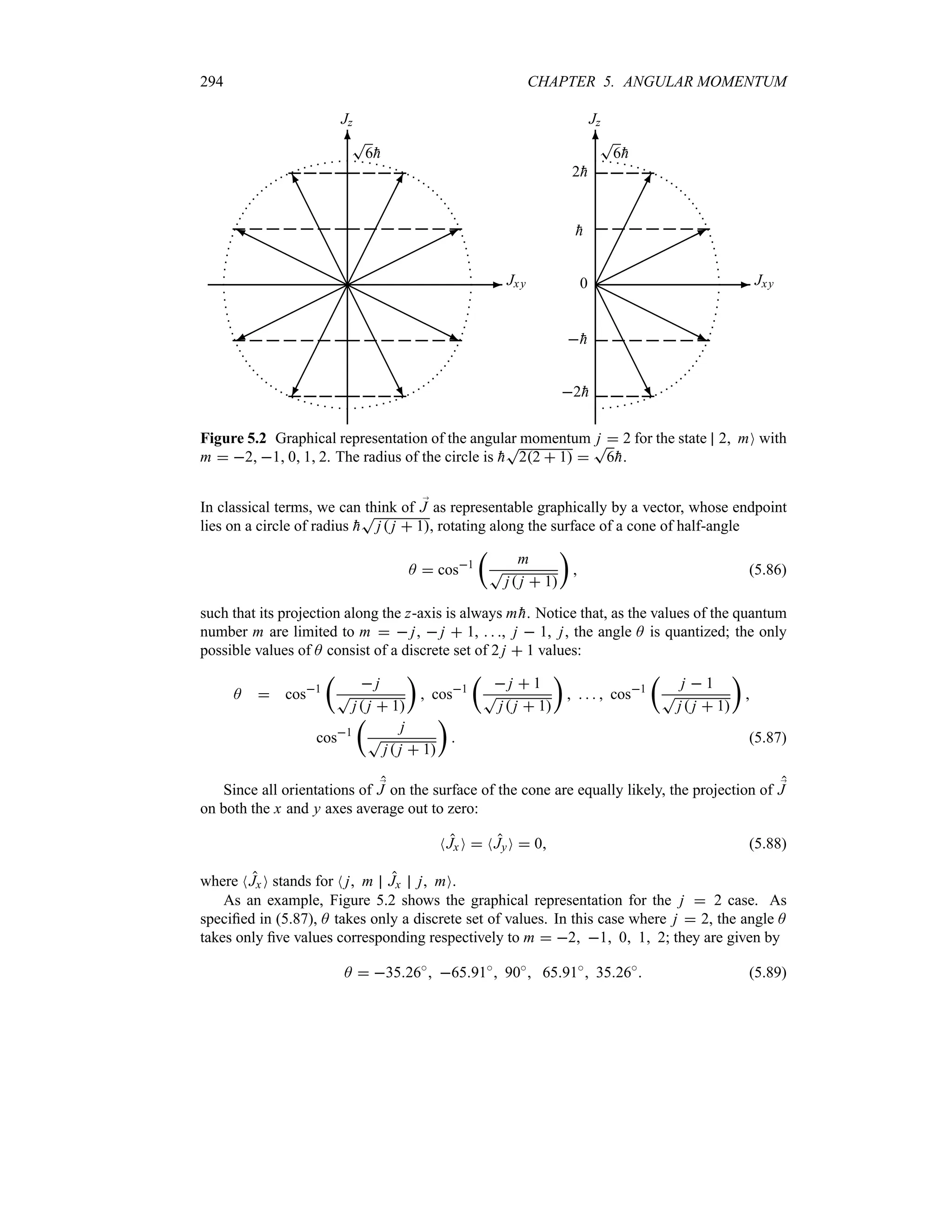
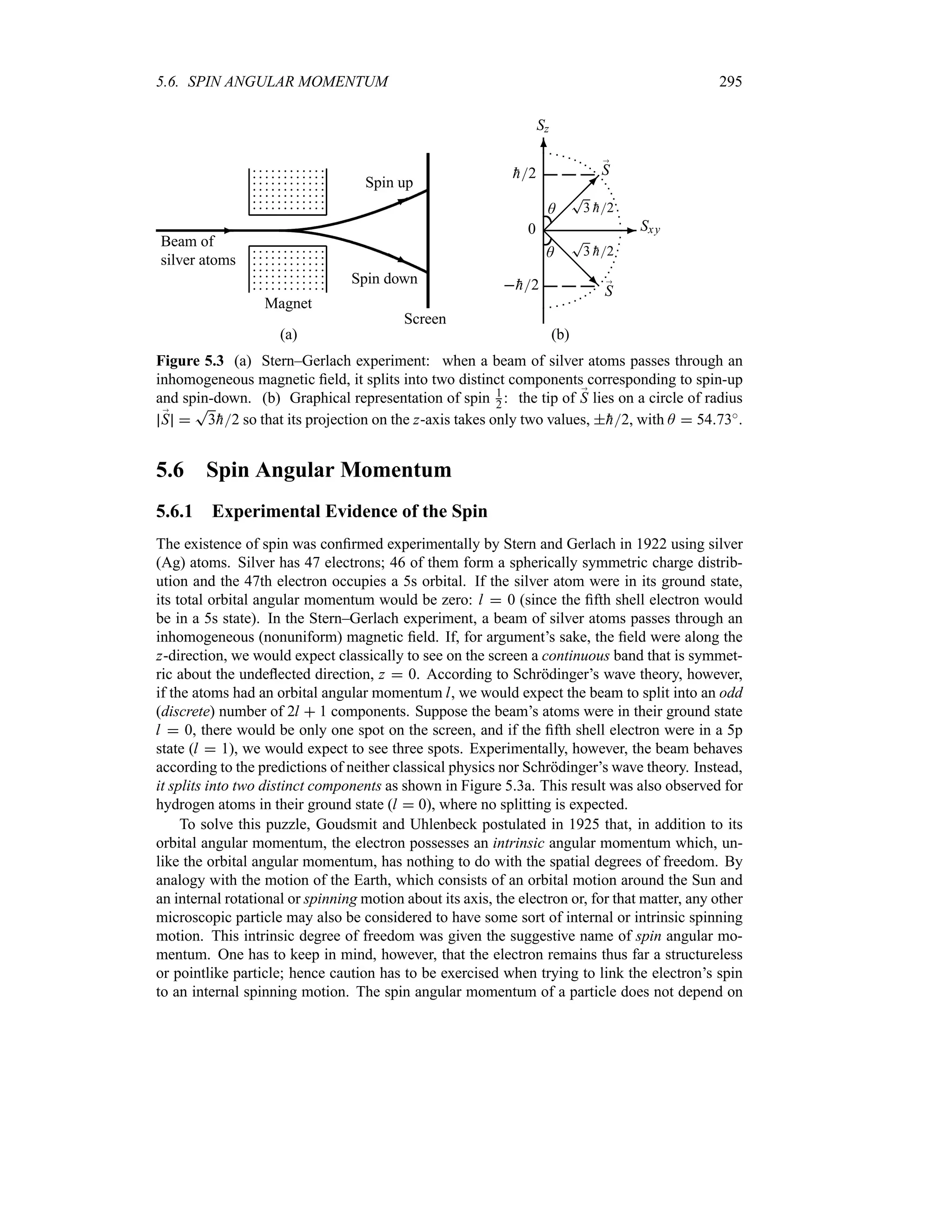
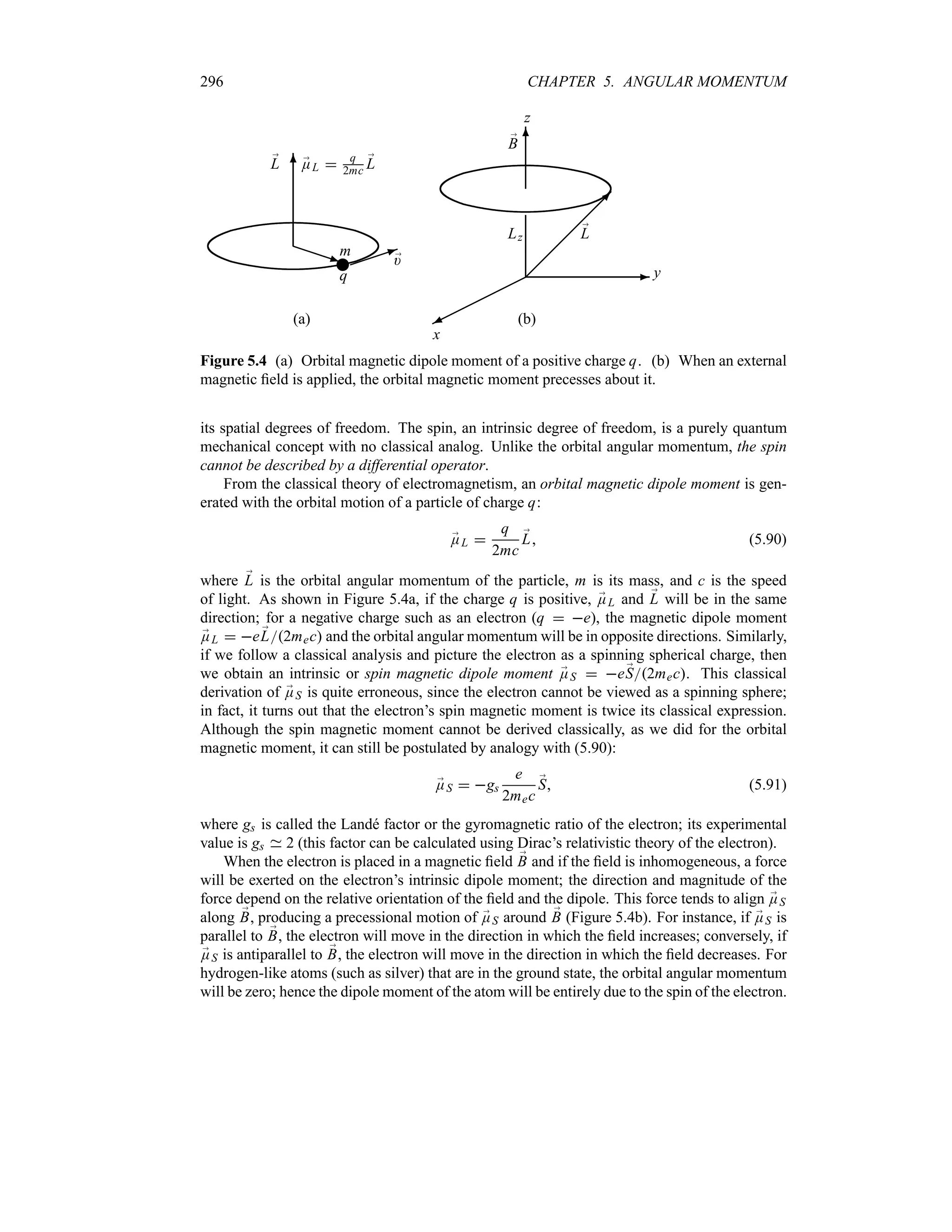
![5.6. SPIN ANGULAR MOMENTUM 297
The atomic beam will therefore deflect according to the orientation of the electron’s spin. Since,
experimentally, the beam splits into two components, the electron’s spin must have only two
possible orientations relative to the magnetic field, either parallel or antiparallel.
By analogy with the orbital angular momentum of a particle, which is characterized by two
quantum numbers—the orbital number l and the azimuthal number ml (with ml l, l 1,
, l 1, l)—the spin angular momentum is also characterized by two quantum numbers, the
spin s and its projection ms on the z-axis (the direction of the magnetic field), where ms s,
s1, , s1, s. Since only two components were observed in the Stern–Gerlach experiment,
we must have 2s 1 2. The quantum numbers for the electron must then be given by s 1
2
and ms 1
2 .
In nature it turns out that every fundamental particle has a specific spin. Some particles
have integer spins s 0, 1, 2 (the pi mesons have spin s 0, the photons have spin s 1,
and so on) and others have half-odd-integer spins s 1
2 , 3
2 , 5
2 (the electrons, protons, and
neutrons have spin s 1
2 , the deltas have spin s 3
2 , and so on). We will see in Chapter 8 that
particles with half-odd-integer spins are called fermions (quarks, electrons, protons, neutrons,
etc.) and those with integer spins are called bosons (pions, photons, gravitons, etc.).
Besides confirming the existence of spin and measuring it, the Stern–Gerlach experiment
offers a number of other important uses to quantum mechanics. First, by showing that a beam
splits into a discrete set of components rather than a continuous band, it provides additional
confirmation for the quantum hypothesis on the discrete character of the microphysical world.
The Stern–Gerlach experiment also turns out to be an invaluable technique for preparing a
quantum state. Suppose we want to prepare a beam of spin-up atoms; we simply pass an
unpolarized beam through an inhomogeneous magnet, then collect the desired component and
discard (or block) the other. The Stern–Gerlach experiment can also be used to determine the
total angular momentum of an atom which, in the case where l / 0, is given by the sum of the
orbital and spin angular momenta: ;
J ;
L ;
S. The addition of angular momenta is covered in
Chapter 7.
5.6.2 General Theory of Spin
The theory of spin is identical to the general theory of angular momentum (Section 5.3). By
analogy with the vector angular momentum ;
J, the spin is also represented by a vector operator
;
S whose components Sx, Sy, Sz obey the same commutation relations as Jx , Jy, Jz:
[Sx Sy] i
hSz [Sy Sz] i
hSx [Sz Sx] i
hSy (5.92)
In addition, ;
S2 and Sz commute; hence they have common eigenvectors:
;
S 2
s msO
h2
ss 1 s msO Sz s msO
hms s msO (5.93)
where ms s, s 1, , s 1, s. Similarly, we have
S s msO
h
S
ss 1 msms 1 s ms 1O (5.94)
where S Sx iSy, and
NS2
x O NS2
yO
1
2
N;
S2
O NS2
z O
h2
2
K
ss 1 m2
s
L
(5.95)](https://image.slidesharecdn.com/zettili-250217213640-909f6141/75/Zettili-Quantum-mechanics-Concept-and-application-pdf-314-2048.jpg)


![300 CHAPTER 5. ANGULAR MOMENTUM
We can verify that the Pauli matrices satisfy the commutation relations
[Jj Jk] 2i jklJl (5.116)
where jkl is the antisymmetric tensor (also known as the Levi–Civita tensor)
jkl
1 if jkl is an even permutation of x y z
1 if jkl is an odd permutation of x y z
0 if any two indices among j kl are equal.
(5.117)
We can condense the relations (5.113), (5.114), and (5.116) into
Jj Jk =j k i
;
l
jklJl (5.118)
Using this relation we can verify that, for any two vectors ;
A and ;
B which commute with ;
J, we
have
;
J ;
A;
J ;
B ;
A ;
BI i ;
J ;
A ;
B (5.119)
where I is the unit matrix. The Pauli matrices are Hermitian, traceless, and have determinants
equal to 1:
J
†
j Jj TrJj 0 detJj 1 j x y z (5.120)
Using the relation Jx Jy iJz along with J2
z I, we obtain
Jx JyJz i I (5.121)
From the commutation relations (5.116) we can show that
ei:Jj I cos : iJj sin : j x y z (5.122)
where I is the unit matrix and : is an arbitrary real constant.
Remarks
Since the spin does not depend on the spatial degrees of freedom, the components Sx, Sy,
Sz of the spin operator commute with all the spatial operators, notably the orbital angular
momentum ;
L, the position and the momentum operators ;
R and ;
P:
[Sj Lk] 0 [Sj Rk] 0 [Sj Pk] 0 j k x y z (5.123)
The total wave function O of a system with spin consists of a product of two parts: a
spatial part O;
r and a spin part s msO:
O OO s msO (5.124)
This product of the space and spin degrees of freedom is not a product in the usual sense,
but a direct or tensor product as discussed in Chapter 7. We will show in Chapter 6 that
the four quantum numbers n, l, ml, and ms are required to completely describe the state
of an electron moving in a central field; its wave function is
nlml ms ;
r Onlml ;
r s msO (5.125)](https://image.slidesharecdn.com/zettili-250217213640-909f6141/75/Zettili-Quantum-mechanics-Concept-and-application-pdf-317-2048.jpg)

![306 CHAPTER 5. ANGULAR MOMENTUM
since Yll cannot be raised further as Yll Ylmmax .
Using the expression (5.134) for L in the spherical coordinates, we can rewrite (5.170) as
follows:
hei
T
2H
v
A
i cot A
w
llAei l
0 (5.171)
which leads to
1
ll
llA
A
l cot A (5.172)
The solution to this differential equation is of the form
llA Cl sinl
A (5.173)
where Cl is a constant to be determined from the normalization condition (5.164) of YllA :
YllA
Cl
T
2H
eil
sinl
A (5.174)
We can ascertain that Cl is given by
Cl
1l
2ll!
U
2l 1!
2
(5.175)
The action of L on YllA is given, on the one hand, by
LYllA
h
T
2lYll1A (5.176)
and, on the other hand, by
LYllA
h
1l
2l l!
U
2l 1!
4H
eil1
sin A1l d
dcos A
[sin A2l
] (5.177)
where we have used the spherical coordinate form (5.134).
Similarly, we can show that the action of Llm
on YllA is given, on the one hand, by
Llm
YllA
hlm
V
2l!l m!
l m!
YlmA (5.178)
and, on the other hand, by
Llm
YllA
hlm 1l
2ll!
U
2l!2l 1!
4H
eim 1
sinm A
dlm
dcos Alm
sin A2l
(5.179)
where m o 0. Equating the previous two relations, we obtain the expression of the spherical
harmonic YlmA for m o 0:
YlmA
1l
2ll!
Vt
2l 1
4H
u
l m!
l m!
eim 1
sinm
A
dlm
dcos Alm
sin A2l
(5.180)](https://image.slidesharecdn.com/zettili-250217213640-909f6141/75/Zettili-Quantum-mechanics-Concept-and-application-pdf-323-2048.jpg)
![5.7. EIGENFUNCTIONS OF ORBITAL ANGULAR MOMENTUM 307
5.7.3 Properties of the Spherical Harmonics
Since the spherical harmonics YlmA are joint eigenfunctions of ;
L2 and Lz and are ortho-
normal (5.164), they constitute an orthonormal basis in the Hilbert space of square-integrable
functions of A and . The completeness relation is given by
l
;
ml
l mONl m 1 (5.181)
or
;
m
NA l mONl m A) )
O
;
m
Y`
l mA)
)
YlmA =cos A cos A)
= )
=A A)
sin A
= )
(5.182)
Let us mention some essential properties of the spherical harmonics. First, the spherical har-
monics are complex functions; their complex conjugate is given by
[YlmA ]`
1m
YlmA (5.183)
We can verify that YlmA is an eigenstate of the parity operator P with an eigenvalue 1l:
PYlmA YlmH A H 1l
YlmA (5.184)
since a spatial reflection about the origin, ;
r ) ;
r, corresponds to r) r, A) H A, and
) H , which leads to Pm
l cos A) Pm
l cos A 1lm Pm
l cos A and eim )
eimH eim 1meim .
We can establish a connection between the spherical harmonics and the Legendre polyno-
mials by simply taking m 0. Then equation (5.180) yields
Yl0A
1l
2ll!
U
2l 1
4H
dl
dcos Al
sin A2l
U
2l 1
4H
Plcos A (5.185)
with
Plcos A
1
2ll!
dl
dcos Al
cos2
A 1l
(5.186)
From the expression of Ylm, we can verify that
Ylm0
U
2l 1
4H
=m 0 (5.187)
The expressions for the spherical harmonics corresponding to l 0 l 1, and l 2 are listed
in Table 5.2.
Spherical harmonics in Cartesian coordinates
Note that YlmA can also be expressed in terms of the Cartesian coordinates. For this, we
need only to substitute
sin A cos
x
r
sin A sin
y
r
cos A
z
r
(5.188)](https://image.slidesharecdn.com/zettili-250217213640-909f6141/75/Zettili-Quantum-mechanics-Concept-and-application-pdf-324-2048.jpg)
![310 CHAPTER 5. ANGULAR MOMENTUM
5.8 Solved Problems
Problem 5.1
(a) Show that Jx Jy
h2[ j j 1m2]2, where Jx
T
NJ2
x O NJxO2 and the same
for Jy.
(b) Show that this relation is consistent with Jx Jy o
h2 NJzO
h2m2.
Solution
(a) First, note that NJxO and NJyO are zero, since
NJxO
1
2
N j m J j mO
1
2
N j m J j mO 0 (5.202)
As for NJ2
x O and NJ2
y O, they are given by
NJ2
x O
1
4
NJ J2
O
1
4
NJ2
J J J J J2
O (5.203)
NJ2
y O
1
4
NJ J2
O
1
4
NJ2
J J J J J2
O (5.204)
Since NJ2
O NJ2
O 0, we see that
NJ2
x O
1
4
NJ J J JO NJ2
y O (5.205)
Using the fact that
NJ2
x O NJ2
y O N ;
J2
O NJ2
z O (5.206)
along with NJ2
x O NJ2
y O, we see that
NJ2
x O NJ2
y O
1
2
[N ;
J2
O NJ2
z O] (5.207)
Now, since j mO is a joint eigenstate of ;
J 2 and Jz with eigenvalues j j 1
h2 and m
h, we
can easily see that the expressions of NJ2
x O and NJ2
y O are given by
NJ2
x O NJ2
y O
1
2
[N ;
J2
O NJ2
z O]
h2
2
K
j j 1 m2
L
(5.208)
Hence Jx Jy is given by
JxJy
T
NJ2
x ONJ2
y O
h2
2
[ j j 1 m2
] (5.209)
(b) Since j o m (because m j j 1 j 1 j), we have
j j 1 m2
o mm 1 m2
m (5.210)
from which we infer that Jx Jy o
h2m2, or
Jx Jy o
h
2
NJzO (5.211)](https://image.slidesharecdn.com/zettili-250217213640-909f6141/75/Zettili-Quantum-mechanics-Concept-and-application-pdf-327-2048.jpg)

![5.8. SOLVED PROBLEMS 319
(a) Find NO L OO.
(b) If Lz were measured what values will one obtain and with what probabilities?
(c) If after measuring Lz we find lz
h, calculate the uncertainties Lx and Ly and
their product LxLy.
Solution
(a) Let us use a lighter notation for OO: OO 1
T
5
1 1O
T
3
5 1 0O 1
T
5
1 1O.
From (5.56) we can write L l mO
h
T
ll 1 mm 1 l m 1O; hence the only
terms that survive in NO L OO are
NO L OO
T
3
5
N1 0 L 1 1O
T
3
5
N1 1 L 1 0O
2
T
6
5
h (5.275)
since N1 0 L 1 1O N1 1 L 1 0O
T
2
h.
(b) If Lz were measured, we will find three values lz
h, 0, and
h. The probability of
finding the value lz
h is
P1 N1 1 OO 2
n
n
n
n
n
1
T
5
N1 1 1 1O
U
3
5
N1 1 1 0O
1
T
5
N1 1 1 1O
n
n
n
n
n
2
1
5
(5.276)
since N1 1 1 0O N1 1 1 1O 0 and N1 1 1 1O 1. Similarly, we can verify
that the probabilities of measuring lz 0 and
h are respectively given by
P0 N1 0 OO 2
n
n
n
n
n
U
3
5
N1 0 1 0O
n
n
n
n
n
2
3
5
(5.277)
P1 N1 1 OO 2
n
n
n
n
n
U
1
5
N1 1 1 1O
n
n
n
n
n
2
1
5
(5.278)
(c) After measuring lz
h, the system will be in the eigenstate lmO 1 1O, that is,
OA Y11A . We need first to calculate the expectation values of Lx , Ly, L2
x, and
L2
y using 1 1O. Symmetry requires that N1 1 Lx 1 1O N1 1 Ly 1 1O 0.
The expectation values of L2
x and L2
y are equal, as shown in (5.60); they are given by
NL2
x O NL2
yO
1
2
[N;
L2
O NL2
z O]
h2
2
K
ll 1 m2
L
h2
2
(5.279)
in this relation, we have used the fact that l 1 and m 1. Hence
Lx
T
NL2
x O
h
T
2
Ly (5.280)
and the uncertainties product Lx Ly is given by
LxLy
T
NL2
xONL2
yO
h2
2
(5.281)](https://image.slidesharecdn.com/zettili-250217213640-909f6141/75/Zettili-Quantum-mechanics-Concept-and-application-pdf-336-2048.jpg)
![320 CHAPTER 5. ANGULAR MOMENTUM
Problem 5.10
Find the angle between the angular momentum l 4 and the z-axis for all possible orientations.
Solution
Since ml 0 1 2 l and the angle between the orbital angular momentum l and the
z-axis is cos Aml ml
T
ll 1 we have
Aml cos1
v
ml
T
ll 1
w
cos1
v
ml
2
T
5
w
(5.282)
hence
A0 cos1
0 90i
(5.283)
A1 cos1
v
1
2
T
5
w
7708i
A2 cos1
v
2
2
T
5
w
6343i
(5.284)
A3 cos1
v
3
2
T
5
w
4787i
A4 cos1
v
4
2
T
5
w
2657i
(5.285)
The angles for the remaining quantum numbers m4 1 2 3 4 can be inferred at once
from the relation
Aml 180i
Aml (5.286)
hence
A1 180i
7708i
10292i
A2 180i
6343i
11657i
(5.287)
A3 180i
4787i
13213i
A4 180i
2657i
15343i
(5.288)
Problem 5.11
Using [X P] i
h, calculate the various commutation relations between the following opera-
tors2
T1
1
4
P2
X2
T2
1
4
X P P X T3
1
4
P2
X2
Solution
The operators T1, T2, and T3 can be viewed as describing some sort of collective vibrations; T3
has the structure of a harmonic oscillator Hamiltonian. The first commutator can be calculated
as follows:
[T1 T2]
1
4
[P2
X2
T2]
1
4
[P2
T2]
1
4
[X2
T2] (5.289)
where, using the commutation relation [X P] i
h, we have
[P2
T2]
1
4
[P2
X P]
1
4
[P2
P X]
1
4
P[P X P]
1
4
[P X P]P
1
4
P[P PX]
1
4
[P P X]P
1
4
P[P X]P
1
4
[P X]P2
1
4
P2
[P X]
1
4
P[P X]P
2N. Zettili and F. Villars, Nucl. Phys., A469, 77 (1987).](https://image.slidesharecdn.com/zettili-250217213640-909f6141/75/Zettili-Quantum-mechanics-Concept-and-application-pdf-337-2048.jpg)
![5.8. SOLVED PROBLEMS 321
i
h
4
P2
i
h
4
P2
i
h
4
P2
i
h
4
P2
i
hP2
(5.290)
[X2
T2]
1
4
[X2
X P]
1
4
[X2
P X]
1
4
X[X X P]
1
4
[X X P]X
1
4
X[X P X]
1
4
[X P X]X
1
4
X2
[X P]
1
4
X[X P]X
1
4
X[X P]X
1
4
[X P]X2
i
h
4
X2
i
h
4
X2
i
h
4
X2
i
h
4
X2
i
hX2
(5.291)
hence
[T1 T2]
1
4
[P2
X2
T2]
1
4
i
hP2
i
hX2
i
hT3 (5.292)
The second commutator is calculated as follows:
[T2 T3]
1
4
[T2 P2
X2
]
1
4
[T2 P2
]
1
4
[T2 X2
] (5.293)
where [T2 P2] and [T2 X2] were calculated in (5.290) and (5.291):
[T2 P2
] i
hP2
[T2 X2
] i
hX2
(5.294)
Thus, we have
[T2 T3]
1
4
i
hP2
i
hX2
i
hT1 (5.295)
The third commutator is
[T3 T1]
1
4
[T3 P2
X2
]
1
4
[T3 P2
]
1
4
[T3 X2
] (5.296)
where
[T3 P2
]
1
4
[P2
P2
]
1
4
[X2
P2
]
1
4
[X2
P2
]
1
4
X[X P2
]
1
4
[X P2
]X
1
4
X P[X P]
1
4
X[X P]P
1
4
P[X P]X
1
4
[X P]P X
i
h
4
2X P 2P X
i
h
2
X P P X (5.297)
[T3 X2
]
1
4
[P2
X2
]
1
4
[X2
X2
]
1
4
[P2
X2
]
i
h
2
X P P X (5.298)
hence
[T3 T1]
1
4
[T3 P2
]
1
4
[T3 X2
]
i
h
8
X P PX
i
h
8
X P P X
i
h
4
X P PX i
hT2 (5.299)
In sum, the commutation relations between T1, T2, and T3 are
[T1 T2] i
hT3 [T2 T3] i
hT1 [T3 T1] i
hT2 (5.300)
These relations are similar to those of ordinary angular momentum, save for the minus sign in
[T1 T2] i
hT3.](https://image.slidesharecdn.com/zettili-250217213640-909f6141/75/Zettili-Quantum-mechanics-Concept-and-application-pdf-338-2048.jpg)

![5.9. EXERCISES 325
the eigenfunction at a later time t is given by
OtO
T
3
2
1Oei E1t
h
1
2
3Oei E3t
h
T
3
4
%
%
#
T
3
0
1
0
$ exp
v
5i0t
2
h
w
1
2
T
12
%
%
#
T
3
0
3
0
$ exp
v
3i0t
2
h
w
(5.322)
5.9 Exercises
Exercise 5.1
(a) Show the following commutation relations:
[Y Ly] 0 [Y Lz] i
hX [Y Lx ] i
hZ
[Z Lz] 0 [Z Lx] i
hY [Z Ly] i
hX
(b) Using a cyclic permutation of xyz, apply the results of (a) to infer expressions for
[X Lx ], [X Ly], and [X Lz].
(c) Use the results of (a) and (b) to calculate [R2 Lx ], [R2 Ly], and [R2 Lx ], where
R2 X2 Y2 Z2.
Exercise 5.2
(a) Show the following commutation relations:
[Py Ly] 0 [Py Lz] i
hPx [Py Lx ] i
hPz
[Pz Lz] 0 [Pz Lx] i
hPy [Pz Ly] i
hPx
(b) Use the results of (a) to infer by means of a cyclic permutation the expressions for
[Px Lx], [Px Ly], and [Px Lz].
(c) Use the results of (a) and (b) to calculate [P2 Lx], [P2 Ly], and [P2 Lz], where
P2 P2
x P2
y P2
z .
Exercise 5.3
If L and R are defined by L Lx i Ly and R X iY, prove the following commu-
tators: (a) [L R] 2
hZ and (b) [L Rb] 0.
Exercise 5.4
If L and R are defined by L Lx i Ly and R X iY, prove the following commu-
tators: (a) [L Z] b
hR, (b) [Lz R]
hR, and (c) [Lz Z] 0.
Exercise 5.5
Prove the following two relations: ;
R ;
L 0 and ;
P ;
L 0.](https://image.slidesharecdn.com/zettili-250217213640-909f6141/75/Zettili-Quantum-mechanics-Concept-and-application-pdf-342-2048.jpg)
![326 CHAPTER 5. ANGULAR MOMENTUM
Exercise 5.6
The Hamiltonian due to the interaction of a particle of spin ;
S with a magnetic field ;
B is given
by H ;
S ;
B where ;
S is the spin. Calculate the commutator [;
S H].
Exercise 5.7
Prove the following relation:
[Lz cos ] i
h sin
where is the azimuthal angle.
Exercise 5.8
Prove the following relation:
[Lz sin2 ] 2i
h
r
sin2
cos2
s
where is the azimuthal angle. Hint: [A BC] B[A C] [A B]C.
Exercise 5.9
Using the properties of J and J, calculate j jO and j mO as functions of the action of
J on the states j mO and j jO, respectively.
Exercise 5.10
Consider the operator A 1
2 Jx Jy Jy Jx.
(a) Calculate the expectation value of A and A
2
with respect to the state j mO.
(b) Use the result of (a) to find an expression for A
2
in terms of: ;
J 4, ;
J2, J2
z , J4
, J4
.
Exercise 5.11
Consider the wave function
OA 3 sin A cos Aei
21 cos2
Ae2i
(a) Write OA in terms of the spherical harmonics.
(b) Write the expression found in (a) in terms of the Cartesian coordinates.
(c) Is OA an eigenstate of ;
L2 or Lz?
(d) Find the probability of measuring 2
h for the z-component of the orbital angular momen-
tum.
Exercise 5.12
Show that Lzcos2 sin2
2i sin cos 2
h2i , where is the azimuthal angle.
Exercise 5.13
Find the expressions for the spherical harmonics Y30A and Y31A ,
Y30A
S
716H5 cos3
A 3 cos A Y31A b
S
2164H sin A5 cos2
A 1ei
in terms of the Cartesian coordinates x y z.
Exercise 5.14
(a) Show that the following expectation values between lmO states satisfy the relations
NLxO NLyO 0 and NL2
x O NL2
yO 1
2
d
ll 1
h2 m2
h2
e
.
(b) Verify the inequality Lx Ly o
h2m2, where Lx
S
NL2
x O NLx O2.](https://image.slidesharecdn.com/zettili-250217213640-909f6141/75/Zettili-Quantum-mechanics-Concept-and-application-pdf-343-2048.jpg)
![5.9. EXERCISES 327
Exercise 5.15
A particle of mass m is fixed at one end of a rigid rod of negligible mass and length R. The
other end of the rod rotates in the xy plane about a bearing located at the origin, whose axis is
in the z-direction.
(a) Write the system’s total energy in terms of its angular momentum L.
(b) Write down the time-independent Schrödinger equation of the system. Hint: In spherical
coordinates, only varies.
(c) Solve for the possible energy levels of the system, in terms of m and the moment of
inertia I mR2.
(d) Explain why there is no zero-point energy.
Exercise 5.16
Consider a system which is described by the state
OA
U
3
8
Y11A
U
1
8
Y10A AY11A
where A is a real constant
(a) Calculate A so that OO is normalized.
(b) Find LOA .
(c) Calculate the expectation values of Lx and ;
L2 in the state OO.
(d) Find the probability associated with a measurement that gives zero for the z-component
of the angular momentum.
(e) Calculate N Lz OO and N L OO where
A
U
8
15
Y11A
U
4
15
Y10A
U
3
15
Y21A
Exercise 5.17
(a) Using the commutation relations of angular momentum, verify the validity of the (Ja-
cobi) identity: [Jx [Jy Jz]] [Jy [Jz Jx]] [Jz [Jx Jy]] 0.
(b)Prove the following identity: [J2
x J2
y ] [J2
y J2
z ] [J2
z J2
x ].
(c) Calculate the expressions of LLYlmA and LLYlmA , and then infer the
commutator [LL LL]YlmA .
Exercise 5.18
Consider a particle whose wave function is given by Ox y z A[x zy z2]r2 A3,
where A is a constant.
(a) Is O an eigenstate of ;
L 2? If yes, what is the corresponding eigenvalue? Is it also an
eigenstate of Lz?
(b) Find the constant A so that O is normalized.
(c) Find the relative probabilities for measuring the various values of Lz and ;
L 2, and then
calculate the expectation values of Lz and ;
L 2.
(d) Calculate L OO and then infer NO L OO.
Exercise 5.19
Consider a system which is in the state
OA
U
2
13
Y33
U
3
13
Y32
U
3
13
Y30
U
3
13
Y32
U
2
13
Y33](https://image.slidesharecdn.com/zettili-250217213640-909f6141/75/Zettili-Quantum-mechanics-Concept-and-application-pdf-344-2048.jpg)
![5.9. EXERCISES 329
(a) Express Ox y z in terms of the spherical harmonics then calculate ;
L2Ox y z and
LzOx y z. Is Ox y z an eigenstate of ;
L2 or Lz?
(b) Calculate LOx y z and NO L OO.
(c) If a measurement of the z-component of the orbital angular momentum is carried out,
find the probabilities corresponding to finding the results 0,
h, and
h.
Exercise 5.25
Consider a system whose wave function is given by
OA
1
2
Y00A
1
T
3
Y11A
1
2
Y11A
1
T
6
Y22A
(a) Is OA normalized?
(b) Is OA an eigenstate of ;
L2 or Lz?
(c) Calculate LOA and NO L OO.
(d) If a measurement of the z-component of the orbital angular momentum is carried out,
find the probabilities corresponding to finding the results 0,
h,
h, and 2
h.
Exercise 5.26
Using the expression of L in spherical coordinates, prove the following two commutators:
[L ei sin A] 0 and [L cos A]
hei sin A.
Exercise 5.27
Consider a particle whose angular momentum is l 1.
(a) Find the eigenvalues and eigenvectors, 1 mx O, of Lx.
(b) Express the state 1 mx 1O as a linear superposition of the eigenstates of Lz. Hint:
you need first to find the eigenstates of Lx and find which of them corresponds to the eigenvalue
mx 1; this eigenvector will be expanded in the z basis.
(c) What is the probability of measuring mz 1 when the particle is in the eigenstate
1 mx 1O? What about the probability corresponding to measuring mz 0?
(d) Suppose that a measurement of the z-component of angular momentum is performed and
that the result mz 1 is obtained. Now we measure the x-component of angular momentum.
What are the possible results and with what probabilities?
Exercise 5.28
Consider a system which is given in the following angular momentum eigenstates l mO:
OO
1
T
7
1 1O A 1 0O
U
2
7
1 1O
where A is a real constant
(a) Calculate A so that OO is normalized.
(b) Calculate the expectation values of Lx, Ly, Lz, and ;
L2 in the state OO.
(c) Find the probability associated with a measurement that gives 1
h for the z-component
of the angular momentum.
(d) Calculate N1 m L2
OO and N1 m L2
OO.](https://image.slidesharecdn.com/zettili-250217213640-909f6141/75/Zettili-Quantum-mechanics-Concept-and-application-pdf-346-2048.jpg)
![330 CHAPTER 5. ANGULAR MOMENTUM
Exercise 5.29
Consider a particle of angular momentum j 32.
(a) Find the matrices representing the operators ;
J2, Jx , Jy, and Jz in the 3
2 mO basis.
(b) Using these matrices, show that Jx , Jy, Jz satisfy the commutator [Jx Jy] i
hJz.
(c) Calculate the mean values of Jx and J2
x with respect to the state
%
%
#
0
0
1
0
$.
(d) Calculate JxJy with respect to the state
%
%
#
0
0
1
0
$
and verify that this product satisfies Heisenberg’s uncertainty principle.
Exercise 5.30
Consider the Pauli matrices
Jx
t
0 1
1 0
u
Jy
t
0 i
i 0
u
Jz
t
1 0
0 1
u
(a) Verify that J2
x J2
y J2
z I, where I is the unit matrix
I
t
1 0
0 1
u
(b) Calculate the commutators [Jx Jy], [Jx Jz], and [Jy Jz].
(c) Calculate the anticommutator Jx Jy JyJx .
(d) Show that eiAJy I cos A iJy sin A, where I is the unit matrix.
(e) Derive an expression for eiAJz by analogy with the one for Jy.
Exercise 5.31
Consider a spin 3
2 particle whose Hamiltonian is given by
H
0
h2
S2
x S2
y
0
h2
S2
z
where 0 is a constant having the dimensions of energy.
(a) Find the matrix of the Hamiltonian and diagonalize it to find the energy levels.
(b) Find the eigenvectors and verify that the energy levels are doubly degenerate.
Exercise 5.32
Find the energy levels of a spin 5
2 particle whose Hamiltonian is given by
H
0
h2
S2
x S2
y
0
h
Sz
where 0 is a constant having the dimensions of energy. Are the energy levels degenerate?](https://image.slidesharecdn.com/zettili-250217213640-909f6141/75/Zettili-Quantum-mechanics-Concept-and-application-pdf-347-2048.jpg)
![5.9. EXERCISES 331
Exercise 5.33
Consider an electron whose spin direction is located in the xy plane.
(a) Find the eigenvalues (call them D1, D2) and eigenstates ( D1O, D2O) of the electron’s
spin operator ;
S.
(b) Assuming that the initial state of the electron is given by
O0O
1
3
D1O
2
T
2
3
D2O
find the probability of obtaining a value of S
h2 after measuring the spin of the electron.
Exercise 5.34
(a) Find the eigenvalues (call them D1, D2) and eigenstates ( D1O, D2O) of the spin operator
;
S of an electron when ;
S is pointing along an arbitrary unit vector ;
n that lies within the yz plane.
(b) Assuming that the initial state of the electron is given by
O0O
1
2
D1O
T
3
2
D2O
find the probability of obtaining a value of S
h2 after measuring the spin of the electron.
Exercise 5.35
Consider a particle of spin 3
2 . Find the matrix for the component of the spin along a unit vector
with arbitrary direction ;
n. Find its eigenvalues and eigenvectors. Hint:
;
n sin A cos ;
i sin A sin ;
j cos A;
k
Exercise 5.36
Show that [Jx Jy Jz] [Jx Jy Jz] i
h
r
J2
x 2J2
y J2
z
s
.
Exercise 5.37
Find the eigenvalues of the operators ;
L
2
and Lz for each of the following states:
(a) Y21A ,
(b) Y32A ,
(c) 1
T
2
d
Y33A Y33A
e
, and
(d) Y40A .
Exercise 5.38
Use the following general relations:
OxO
1
T
2
vn
n
n
n
1
2
1
2
n
n
n
n
1
2
1
2
w
OyO
1
T
2
vn
n
n
n
1
2
1
2
i
n
n
n
n
1
2
1
2
w
to verify the following eigenvalue equations:
Sx OxO
h
2
Ox O and Sy OyO
h
2
n
nOy
m](https://image.slidesharecdn.com/zettili-250217213640-909f6141/75/Zettili-Quantum-mechanics-Concept-and-application-pdf-348-2048.jpg)


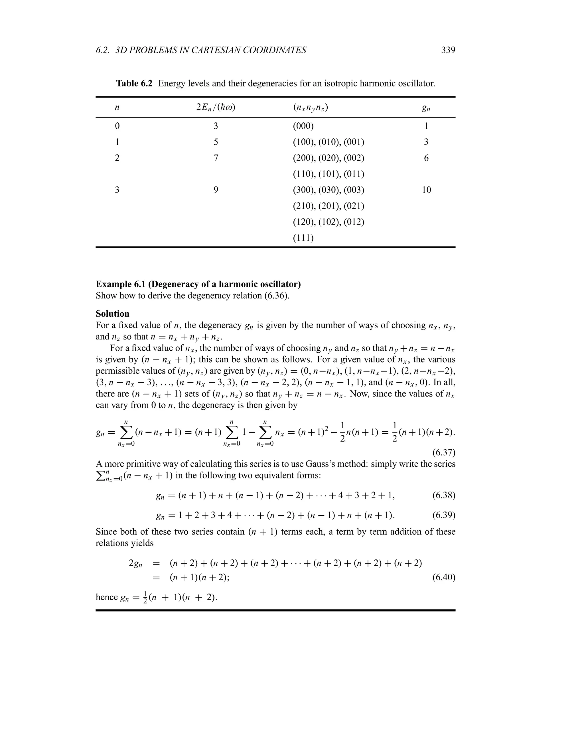
![340 CHAPTER 6. THREE-DIMENSIONAL PROBLEMS
6.3 3D Problems in Spherical Coordinates
6.3.1 Central Potential: General Treatment
In this section we study the structure of the Schrödinger equation for a particle of mass1 M
moving in a spherically symmetric potential
V;
r Vr (6.41)
which is also known as the central potential.
The time-independent Schrödinger equation for this particle, of momentum i
h ;
V and po-
sition vector ;
r, is
h2
2M
V2
Vr
O;
r EO;
r (6.42)
Since the Hamiltonian is spherically symmetric, we are going to use the spherical coordinates
r A which are related to their Cartesian counterparts by
x r sin A cos y r sin A sin z r cos A (6.43)
The Laplacian V2 separates into a radial part V2
r and an angular part V2
P as follows (see Chapter
5):
V2
V2
r
1
h2r2
V2
P
1
r2
r
t
r2
r
u
1
h2r2
;
L
2
1
r
2
r2
r
1
h2r2
;
L
2
(6.44)
where ;
L is the orbital angular momentum with
;
L2
h2
v
1
sin A
A
t
sin A
A
u
1
sin2
A
2
2
w
(6.45)
In spherical coordinates the Schrödinger equation therefore takes the form
h2
2M
1
r
2
r2
r
1
2Mr2
;
L2
Vr
O;
r EO;
r (6.46)
The first term of this equation can be viewed as the radial kinetic energy
h2
2M
1
r
2
r2
r
P2
r
2M
(6.47)
since the radial momentum operator is given by the Hermitian form2
Pr
1
2
vt
;
r
r
u
;
P ;
P
t
;
r
r
uw
i
h
t
r
1
r
u
k i
h
1
r
r
r (6.48)
1Throughout this section we will designate the mass of the particle by a capital M to avoid any confusion with the
azimuthal quantum number m.
2Note that we can show that the commutator between the position operator, r, and the radial momentum operator,
pr , is given by: [r pr ] i
h (the proof is left as an exercise).](https://image.slidesharecdn.com/zettili-250217213640-909f6141/75/Zettili-Quantum-mechanics-Concept-and-application-pdf-357-2048.jpg)
![6.3. 3D PROBLEMS IN SPHERICAL COORDINATES 341
The second term ;
L22Mr2 of (6.46) can be identified with the rotational kinetic energy, for
this term is generated from a “pure” rotation of the particle about the origin (i.e., no change in
the radial variable r, where Mr2 is its moment of inertia with respect to the origin).
Now, since ;
L2 as shown in (6.45) does not depend on r, it commutes with both Vr and
the radial kinetic energy; hence it also commutes with the Hamiltonian H. In addition, since
Lz commutes with ;
L2, the three operators H, ;
L2, and Lz mutually commute:
[H ;
L2
] [H Lz] 0 (6.49)
Thus H, ;
L2, and Lz have common eigenfunctions. We have seen in Chapter 5 that the simulta-
neous eigenfunctions of ;
L2 and Lz are given by the spherical harmonics YlmA :
;
L2
YlmA ll 1
h2
YlmA (6.50)
LzYlmA m
hYlmA (6.51)
Since the Hamiltonian in (6.46) is a sum of a radial part and an angular part, we can look for
solutions that are products of a radial part and an angular part, where the angular part is simply
the spherical harmonic YlmA :
O;
r N;
r nlmO Onlmr A RnlrYlmA (6.52)
Note that the orbital angular momentum of a system moving in a central potential is conserved,
since, as shown in (6.49), it commutes with the Hamiltonian.
The radial wave function Rnlr has yet to be found. The quantum number n is introduced
to identify the eigenvalues of H:
H nlmO En nlmO (6.53)
Substituting (6.52) into (6.46) and using the fact that Onlmr A is an eigenfunction of ;
L2
with eigenvalue ll 1
h2, then dividing through by RnlrYlmA and multiplying by 2Mr2,
we end up with an equation where the radial and angular degrees of freedom are separated:
v
h2 r
Rnl
2
r2
r Rnl 2Mr2
Vr E
w
;
L2YlmA
YlmA
0 (6.54)
The terms inside the first square bracket are independent of A and and those of the second
are independent of r. They must then be separately equal to constants and their sum equal to
zero. The second square bracket is nothing but (6.50), the eigenvalue equation of ;
L2; hence it
is equal to ll 1
h2. As for the first bracket, it must be equal to ll 1
h2; this leads to an
equation known as the radial equation for a central potential:
h2
2M
d2
dr2
r Rnlr
Vr
ll 1
h2
2Mr2
r Rnlr En r Rnlr (6.55)
Note that (6.55), which gives the energy levels of the system, does not depend on the azimuthal
quantum number m. Thus, the energy En is 2l1-fold degenerate. This is due to the fact that,](https://image.slidesharecdn.com/zettili-250217213640-909f6141/75/Zettili-Quantum-mechanics-Concept-and-application-pdf-358-2048.jpg)
![342 CHAPTER 6. THREE-DIMENSIONAL PROBLEMS
for a given l, there are 2l 1 different eigenfunctions Onlm (i.e., Onl l, Onl l1, , Onl l1,
Onl l) which correspond to the same eigenenergy En. This degeneracy property is peculiar to
central potentials.
Note that (6.55) has the structure of a one-dimensional equation in r,
h2
2M
d2Unlr
dr2
Vr
ll 1
h2
2Mr2
Unlr EnUnlr (6.56)
or
h2
2M
d2Unlr
dr2
Veff rUnlr EnUnlr (6.57)
whose solutions give the energy levels of the system. The wave function Unlr is given by
Unlr r Rnlr (6.58)
and the potential by
Veff r Vr
ll 1
h2
2Mr2
(6.59)
which is known as the effective or centrifugal potential, where Vr is the central potential
and ll 1
h22Mr2 is a repulsive or centrifugal potential, associated with the orbital angular
momentum, which tends to repel the particle away from the center. As will be seen later, in the
case of atoms, Vr is the Coulomb potential resulting from the attractive forces between the
electrons and the nucleus. Notice that although (6.57) has the structure of a one-dimensional
eigenvalue equation, it differs from the one-dimensional Schrödinger equation in one major
aspect: the variable r cannot have negative values, for it varies from r 0 to r *. We
must therefore require the wave function Onlmr A to be finite for all values of r between 0
and *, notably for r 0. But if Rnl0 is finite, r Rnlr must vanish at r 0, i.e.,
lim
r0
[r Rnlr] Unl0 0 (6.60)
Thus, to make the radial equation (6.57) equivalent to a one-dimensional eigenvalue problem,
we need to assume that the particle’s potential is given by the effective potential Veff r for
r 0 and by an infinite potential for r n 0.
For the eigenvalue equation (6.57) to describe bound states, the potential Vr must be
attractive (i.e., negative) because ll 1
h22Mr2 is repulsive. Figure 6.1 shows that, as l
increases, the depth of Veff r decreases and its minimum moves farther away from the origin.
The farther the particle from the origin, the less bound it will be. This is due to the fact that as
the particle’s angular momentum increases, the particle becomes less and less bound.
In summary, we want to emphasize the fact that, for spherically symmetric potentials, the
Schrödinger equation (6.46) reduces to a trivial angular equation (6.50) for ;
L2 and to a one-
dimensional radial equation (6.57).
Remark
When a particle has orbital and spin degrees of freedom, its total wave function O consists
of a product of two parts: a spatial part, O;
r, and a spin part, s msO; that is, O
OO s msO. In the case of an electron moving in a central field, besides the quantum numbers](https://image.slidesharecdn.com/zettili-250217213640-909f6141/75/Zettili-Quantum-mechanics-Concept-and-application-pdf-359-2048.jpg)
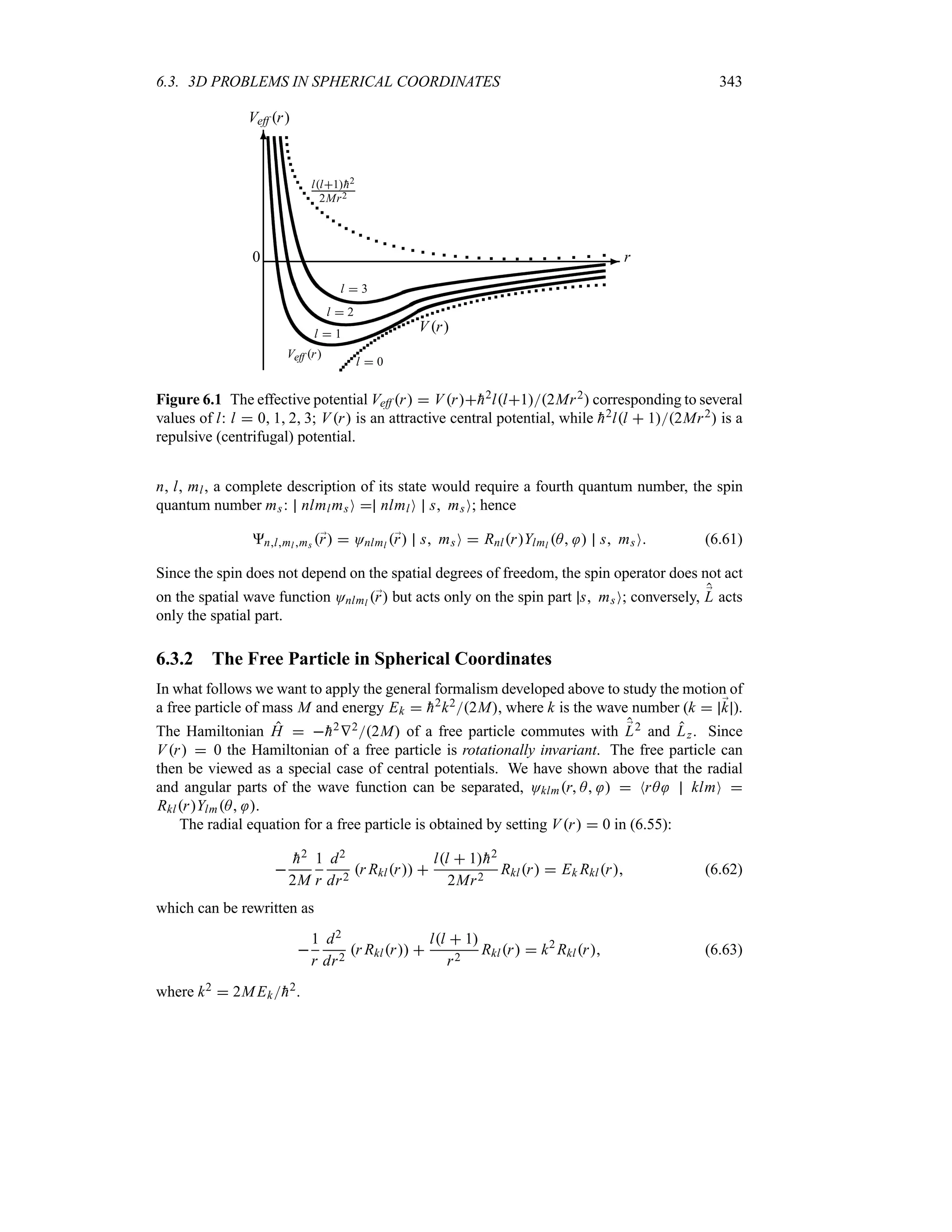
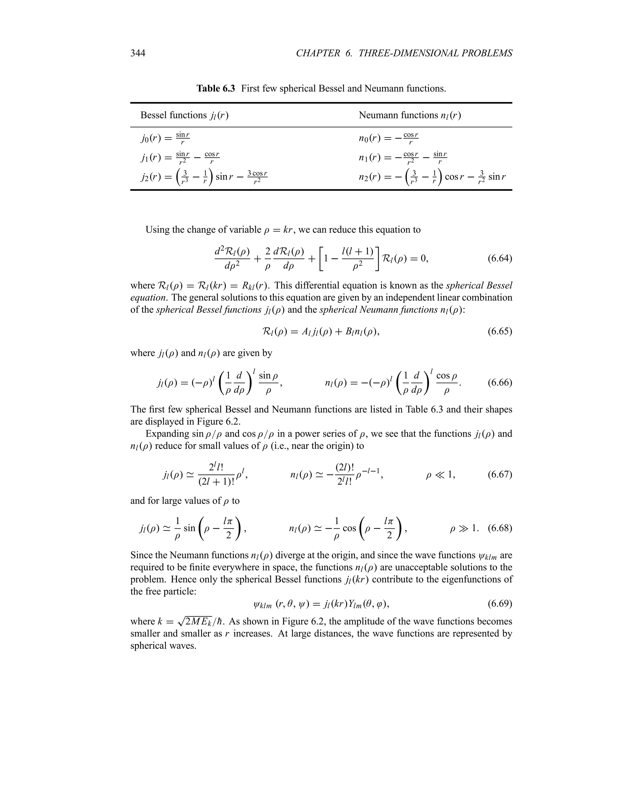
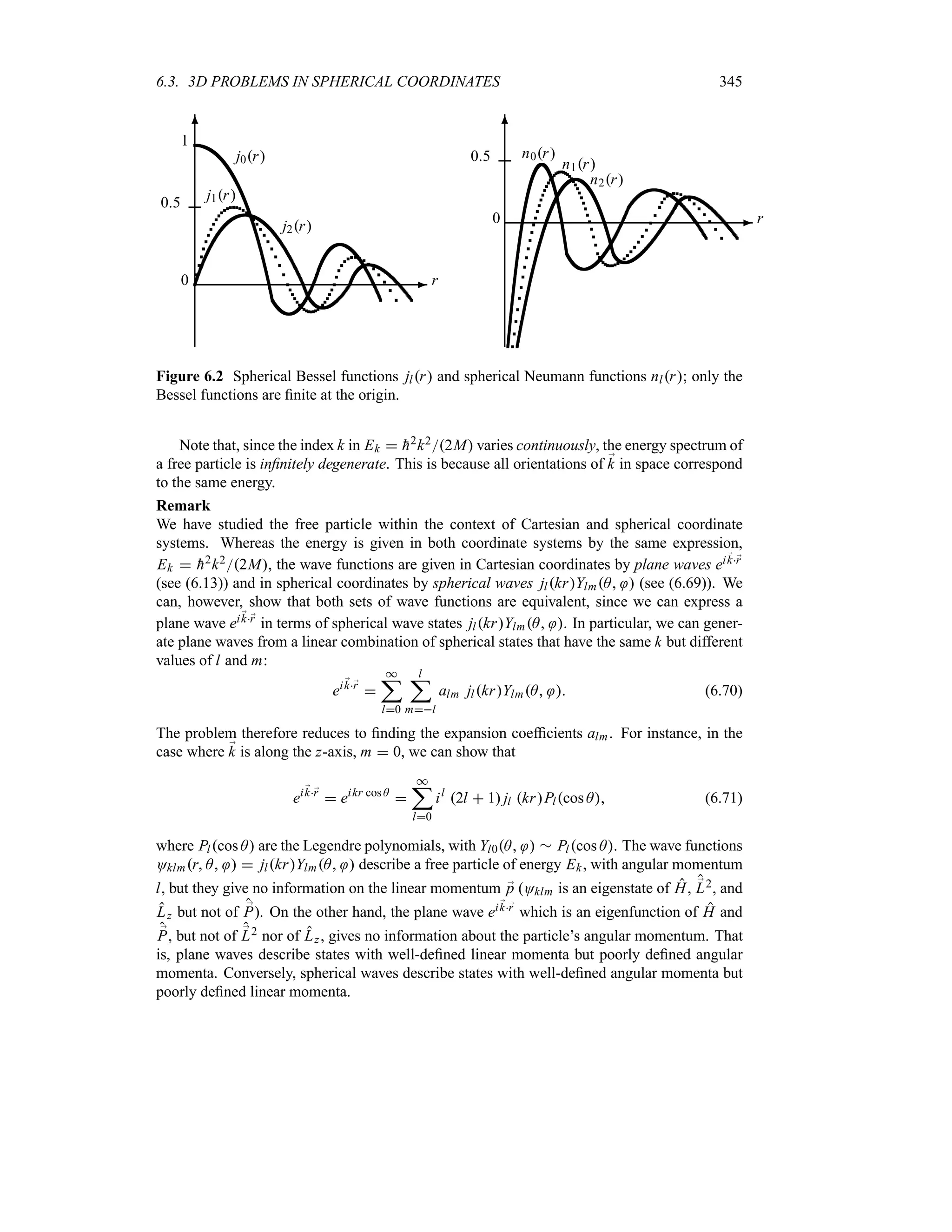

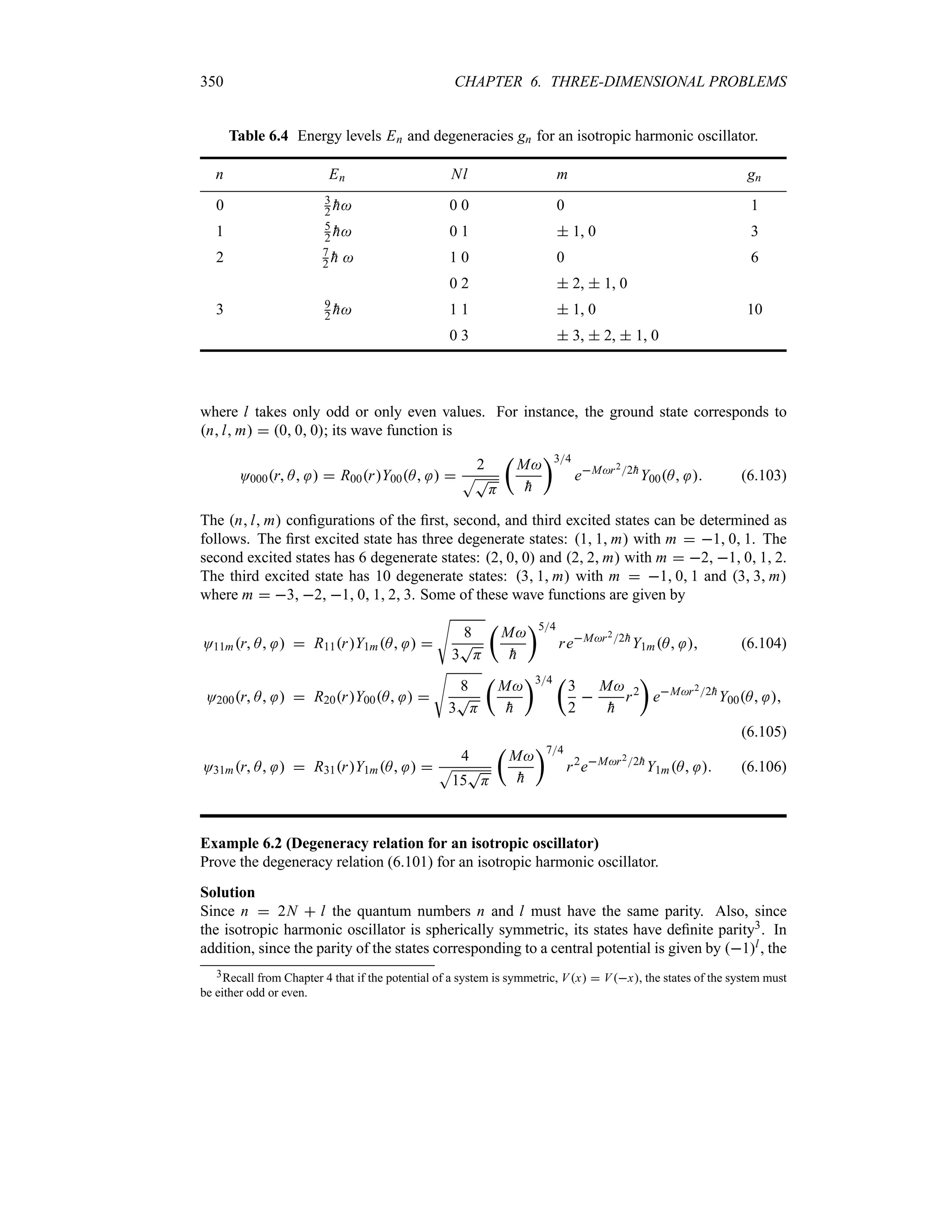
![358 CHAPTER 6. THREE-DIMENSIONAL PROBLEMS
Table 6.5 First few Laguerre polynomials and associated Laguerre polynomials.
Laguerre polynomials Lkr Associated Laguerre polynomials LN
k r
L0 1
L1 1 r L1
1 1
L2 2 4r r2 L1
2 4 2r, L2
2 2
L3 6 18r 9r2 r3 L1
3 18 18r 3r2, L2
3 18 6r, L3
3 6
L4 24 96r 72r2 16r3 r4 L1
4 96 144r 48r2 4r3
L2
4 144 96r 12r2, L3
4 24r 96, L4
4 24
L5 120 600r 600r2 200r3 L1
5 600 1200r 600r2 100r3 5r4
25r4 r5 L2
5 1200 1200r 300r2 20r3
L3
5 1200 600r 60r2, L4
5 600 120r
L5
5 120
The first few Laguerre polynomials are listed in Table 6.5.
We can verify that Lkr and LN
k r satisfy the following differential equations:
r
d2Lkr
dr2
1 r
dLkr
dr
kLkr 0 (6.161)
r
d2LN
k r
dr2
N 1 r
dLN
k r
dr
k NLN
k r 0 (6.162)
This last equation is identical to the hydrogen atom radial equation (6.134). The proof goes as
follows. Using a change of variable
I 2Dr 2
T
2EE
h
r (6.163)
along with the fact that a0
h2Ee2 (Bohr radius), we can show that (6.134) reduces to
I
d2gI
dI2
[2l 1 1 I]
dgI
dI
[n l 2l 1] gI 0 (6.164)
where f r gI. In deriving (6.164), we have used the fact that 1Da0 n (see (6.148)).
Note that equations (6.162) and (6.164) are identical; the solutions to (6.134) are thus given by
the associated Laguerre polynomials L2l1
nl 2Dr.
The radial wave function of the hydrogen atom is then given by
Rnlr Nnl
t
2r
na0
ul
erna0 L2l1
nl
t
2r
na0
u
(6.165)
where Nnl is a constant obtained by normalizing the radial function Rnlr:
= *
0
r2
R2
nlr dr 1 (6.166)](https://image.slidesharecdn.com/zettili-250217213640-909f6141/75/Zettili-Quantum-mechanics-Concept-and-application-pdf-375-2048.jpg)
![6.3. 3D PROBLEMS IN SPHERICAL COORDINATES 359
Table 6.6 The first few radial wave functions Rnlr of the hydrogen atom.
R10r 2a
32
0 era0 R21r 1
T
6a3
0
r
2a0
er2a0
R20r 1
T
2a3
0
r
1 r
2a0
s
er2a0 R31r 8
9
T
6a3
0
r
1 r
6a0
s r
r
3a0
s
er3a0
R30r 2
3
T
3a3
0
t
1 2r
3a0
2r2
27a2
0
u
er3a0 R32r 4
9
T
30a3
0
r
r
3a0
s2
er3a0
Using the normalization condition of the associated Laguerre functions
= *
0
eI
I2l
K
L2l1
nl I
L2
I2
dI
2n [n l!]3
n l 1!
(6.167)
where I 2Dr 2rna0, we can show that Nnl is given by
Nnl
t
2
na0
u32
V
n l 1!
2n[n l!]3
(6.168)
The wave functions of the hydrogen atom are given by
Onlmr A RnlrYlmA (6.169)
where the radial functions Rnlr are
Rnlr
t
2
na0
u32
V
n l 1!
2n[n l!]3
t
2r
na0
ul
erna0 L2l1
nl
t
2r
na0
u
(6.170)
The first few radial wave functions are listed in Table 6.6; as shown in (6.155) and (6.158),
they are identical with those obtained from a straightforward construction of Rnlr. The shapes
of some of these radial functions are plotted in Figure 6.3.
(e) Properties of the radial wave functions of hydrogen
The radial wave functions of the hydrogen atom behave as follows (see Figure 6.3):
They behave like rl for small r.
They decrease exponentially at large r, since L2l1
nl is dominated by the highest power,
rnl1.
Each function Rnlr has n l 1 radial nodes, since L2l1
nl I is a polynomial of degree
n l 1.](https://image.slidesharecdn.com/zettili-250217213640-909f6141/75/Zettili-Quantum-mechanics-Concept-and-application-pdf-376-2048.jpg)
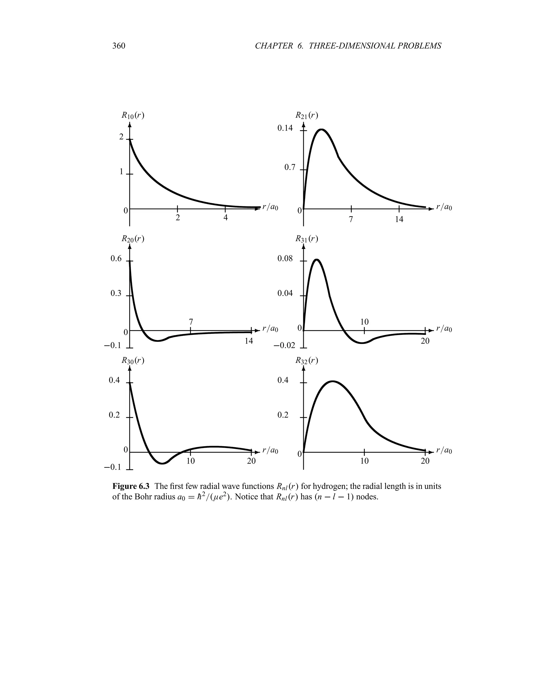
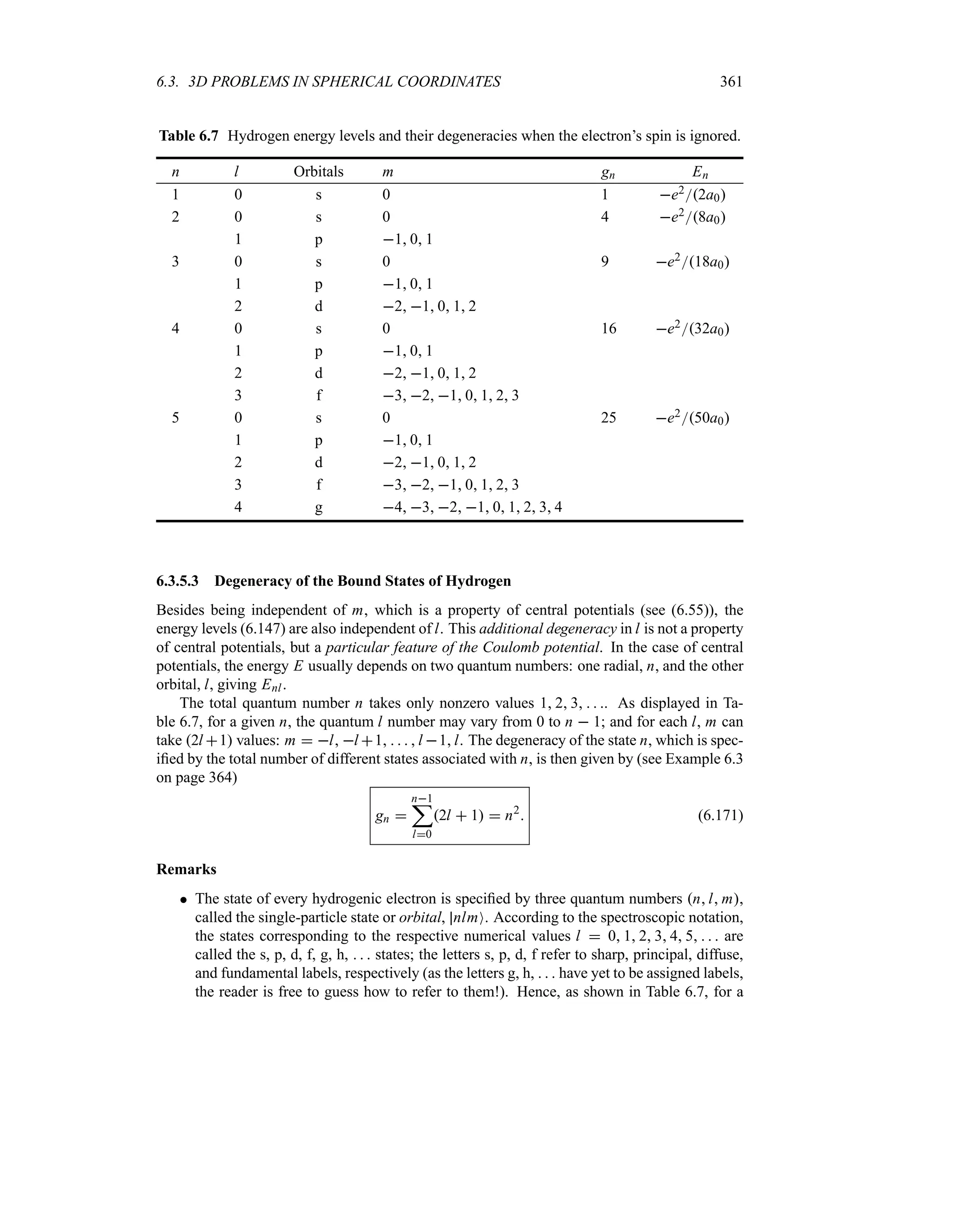

![6.3. 3D PROBLEMS IN SPHERICAL COORDINATES 365
6.3.6 Effect of Magnetic Fields on Central Potentials
As discussed earlier (6.55), the energy levels of a particle in a central potential do not depend
on the azimuthal quantum number m. This degeneracy can be lifted if we place the particle in
a uniform magnetic field ;
B (if ;
B is uniform, its spatial derivatives vanish).
6.3.6.1 Effect of a Magnetic Field on a Charged Particle
Consider a particle of mass E and charge q which, besides moving in a central potential Vr,
is subject to a uniform magnetic field ;
B.
From the theory of classical electromagnetism, the vector potential corresponding to a uni-
form magnetic field may be written as ;
A 1
2 ;
B ;
r since, using the relation ;
V ;
C ;
D
;
C ;
V ;
D ;
D ;
V ;
C ;
D ;
V ;
C ;
C ;
V ;
D, we have
;
V ;
A
1
2
;
V ;
B ;
r
1
2
K
;
B ;
V ;
r ;
B ;
V;
r
L
1
2
K
3 ;
B ;
B
L
;
B (6.193)
where we have used ;
V ;
B 0, ;
r ;
V ;
B 0, ;
V ;
r 3, and ;
B ;
V;
r ;
B. When the charge
is placed in a magnetic field ;
B, its linear momentum becomes ;
p ;
p qc ;
A, where c is the
speed of light. The Hamiltonian of the particle is thus given by (see (6.124))
H
1
2E
r
;
p
q
c
;
A
s2
Vr H0
q
2Ec
r
;
p ;
A ;
A ;
p
s
q2
2Ec2
;
A2
(6.194)
where H0 ;
p 22E Vr is the Hamiltonian of the particle when the magnetic field ;
B is
not present. The term ;
p ;
A can be calculated by analogy with the commutator [p Fx]
i
hdFxdx:
;
p ;
A OO i
h ;
V ;
A OO i
h ;
A ;
V OO i
h ;
V ;
A OO ;
A ;
p OO (6.195)
We see that, whenever ;
V ;
A 0 is valid (the Coulomb gauge), ;
A ;
p is equal to ;
p ;
A:
;
p ;
A ;
A ;
p i
h ;
V ;
A 0 ;
A ;
p ;
p ;
A (6.196)
On the other hand, since ;
A 1
2 ;
B ;
r, we have
;
A ;
p
1
2
;
B ;
r ;
p
1
2
;
B ;
r ;
p
1
2
;
B ;
L (6.197)
where ;
L is the orbital angular momentum operator of the particle. Now, a combination of
(6.196) and (6.197) leads to ;
p ;
A ;
A ;
p 1
2
;
B ;
L which, when inserted in the Hamiltonian
(6.194), yields
H H0
q
Ec
;
A ;
p
q2
2Ec2
;
A2
H0
q
2Ec
;
B ;
L
q2
2Ec2
;
A 2
H0 ;
EL ;
B
q2
2Ec2
;
A 2
(6.198)
where
;
EL
q
2Ec
;
L
EB
h
;
L (6.199)
is called the orbital magnetic dipole moment of the charge q and EB q
h2Ec is known as
the Bohr magneton; as mentioned in Chapter 5, ;
EL is due to the orbiting motion of the charge](https://image.slidesharecdn.com/zettili-250217213640-909f6141/75/Zettili-Quantum-mechanics-Concept-and-application-pdf-382-2048.jpg)
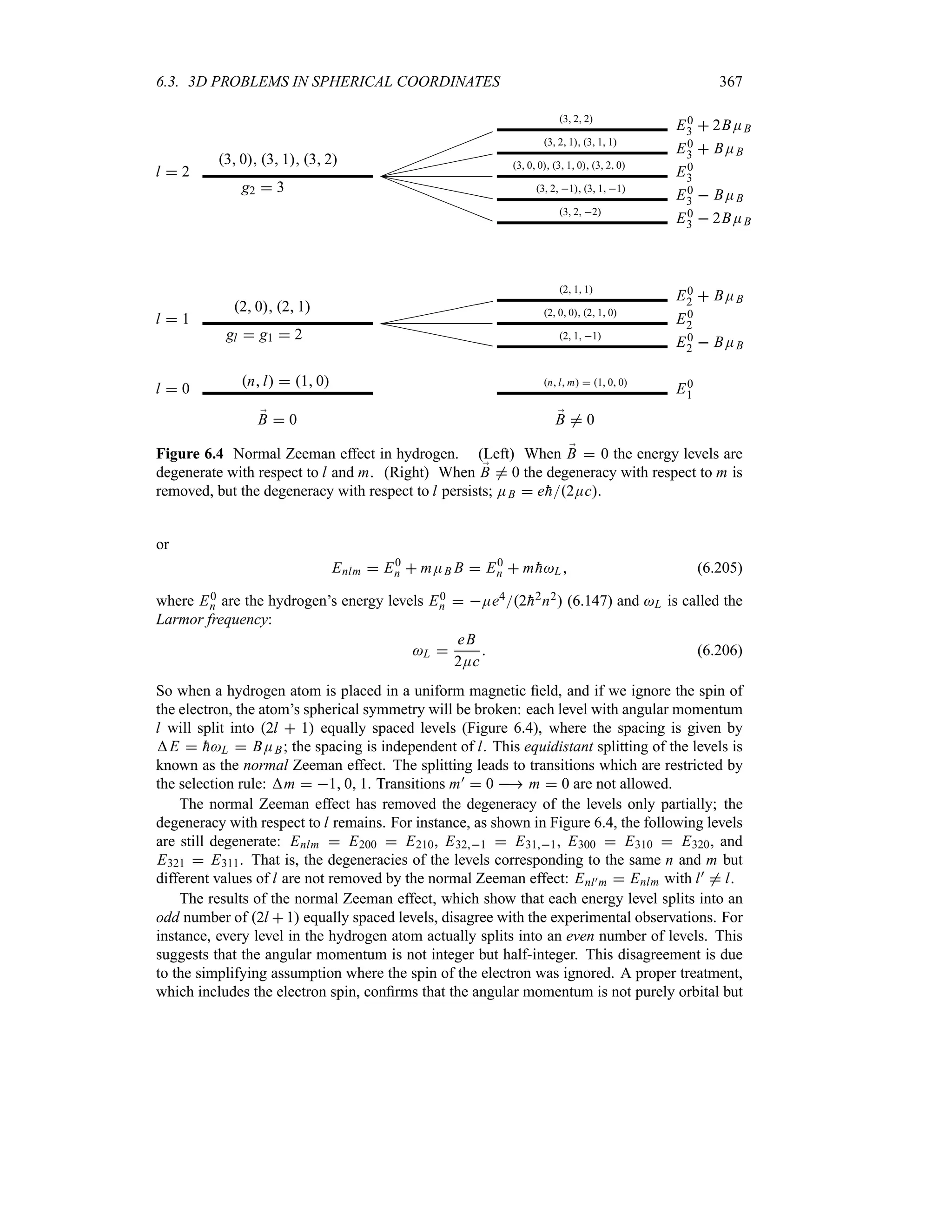

![374 CHAPTER 6. THREE-DIMENSIONAL PROBLEMS
since n 2. We see that
E1l 7 E2l 0 (6.251)
(c) Since the probability of finding the electron in the sphere of radius a is equal to 1, the
probability of finding it in a sphere of radius a2 is equal to 12.
As for the probability of finding the electron in the spherical shell between r a and
r 3a2, it is equal to zero, since the electron cannot tunnel through the infinite potential from
r a to r a.
Problem 6.5
Find the l 0 energy and wave function of a particle of mass m that is subject to the following
central potential Vr
|
0 a r b
* elsewhere
Solution
This particle moves between two concentric, hard spheres of radii r a and r b. The l 0
radial equation between a r b can be obtained from (6.57):
d2Un0r
dr2
k2
Un0r 0 (6.252)
where Un0r r Rn0r and k2 2mE
h2. Since the solutions of this equation must satisfy
the condition Un0a 0, we may write
Un0r A sin[kr a] (6.253)
the radial wave function is zero elsewhere, i.e., Un0r 0 for 0 r a and r b.
Moreover, since the radial function must vanish at r b, Un0b 0, we have
A sin[kb a] 0 kb a nH n 1 2 3 (6.254)
Coupled with the fact that k2 2mE
h2, this condition leads to the energy
En
h2k2
2m
H2
h2
2ma b2
n 1 2 3 (6.255)
We can normalize the radial function (6.253) to obtain the constant A:
1
= b
a
r2
R2
n0rdr
= b
a
U2
n0rdr A2
= b
a
sin2
[kr a] dr
A2
2
= b
a
1 cos[2kr a] dr
b a
2
A2
(6.256)
hence A
T
2b a. Since kn nHb a the normalized radial function is given by
Rn0r
1
r
Un0r
T
2
ba
1
r sin[nHra
ba ] a r b
0 elsewhere
(6.257)](https://image.slidesharecdn.com/zettili-250217213640-909f6141/75/Zettili-Quantum-mechanics-Concept-and-application-pdf-391-2048.jpg)
![6.5. SOLVED PROBLEMS 375
To obtain the total wave function Onlm;
r, we need simply to divide the radial function by a
1
T
4H factor, because in this case of l 0 the wave function On00r depends on no angular
degrees of freedom, it depends only on the radius:
On00r
1
T
4H
Rn0r
T
2
4Hba
1
r sin[nHra
ba ] a r b
0 elsewhere
(6.258)
Problem 6.6
(a) For the following cases, calculate the value of r at which the radial probability density
of the hydrogen atom reaches its maximum: (i) n 1, l 0, m 0; (ii) n 2, l 1, m 0;
(iii) l n 1, m 0.
(b) Compare the values obtained with the Bohr radius for circular orbits.
Solution
(a) Since the radial wave function for n 1 and l 0 is R10r 2a
32
0 era0 , the
probability density is given by
P10r r2
R10r 2
4
a3
0
r2
e2ra0 (6.259)
(i) The maximum of P10r occurs at r1:
d P10r
dr
n
n
n
n
rr1
0 2r1
2r2
1
a0
0 r1 a0 (6.260)
(ii) Similarly, since R21r 12
T
6a
52
0 rer2a0 , we have
P21r r2
R21r 2
1
24a5
0
r4
era0 (6.261)
The maximum of the probability density is given by
d P21r
dr
n
n
n
n
rr2
0 4r3
2
r4
2
a0
0 r2 4a0 (6.262)
(iii) The radial function for l n 1 can be obtained from (6.170):
Rnn1r
t
2
na0
u32
1
S
2n[2n 1!]3
t
2r
na0
un1
erna0 L2n1
2n1
t
2r
na0
u
(6.263)
From (6.159) and (6.160) we can verify that the associated Laguerre polynomial L2n1
2n1 is a con-
stant, L2n1
2n1 y 2n 1!. We can thus write Rnn1r as Rnn1r Anrn1erna0 ,
where An is a constant. Hence the probability density is given by
Pnn1r r2
Rnn1r 2
A2
nr2n
e2rna0 (6.264)
The maximum of the probability density is given by
d Pnn1r
dr
n
n
n
n
rrn
0 2nr2n1
n
2r2n
n
na0
0 rn n2
a0 (6.265)](https://image.slidesharecdn.com/zettili-250217213640-909f6141/75/Zettili-Quantum-mechanics-Concept-and-application-pdf-392-2048.jpg)

![6.5. SOLVED PROBLEMS 377
Problem 6.8
The operators associated with the radial component of the momentum pr and the radial coordi-
nate r are denoted by Pr and R, respectively. Their actions on a radial wave function Or are
given by Pr O;
r i
h1rrrO;
r and RO;
r rO;
r.
(a) Find the commutator [Pr R] and Pr r, where r
T
NR2O NRO2 and
Pr
T
NP2
r O NPr O2.
(b) Show that P2
r
h2r2r2r.
Solution
(a) Since RO;
r rO;
r and
Pr O;
r i
h
1
r
r
rO;
r i
h
1
r
O;
r i
h
O;
r
r
(6.269)
and since
Pr RO;
r i
h
1
r
r
r
r2
O;
r
s
2i
hO;
r i
hr
O;
r
r
(6.270)
the action of the commutator [Pr R] on a function O;
r is given by
[Pr R]O;
r i
h
v
1
r
r
r R
w
O;
r i
h
1
r
r
r
r2
O;
r
s
i
h
r
rO;
r
2i
hO;
r i
hr
O;
r
r
i
hO;
r i
hr
O;
r
r
i
hO;
r (6.271)
Thus, we have
[Pr R] i
h (6.272)
Using the uncertainty relation for a pair of operators A and B, AB o 1
2 N[A B]O , we can
write
Pr r o
1
2
n
n
n
'
[Pr R]
(n
n
n (6.273)
or
Pr r o
h
2
(6.274)
(b) The action of P2
r on O;
r gives
P2
r O;
r
h2 1
r
r
v
r
1
r
r
rO
w
h2 1
r
2
r2
rO;
r (6.275)
hence
P2
r
h2 1
r
2
r2
r (6.276)
Problem 6.9
Find the number of s bound states for a particle of mass m moving in a delta potential Vr
V0=r a where V0 0. Discuss the existence of bound states in terms of the size of a.
Find the normalized wave function of the bound state(s).](https://image.slidesharecdn.com/zettili-250217213640-909f6141/75/Zettili-Quantum-mechanics-Concept-and-application-pdf-394-2048.jpg)
![6.5. SOLVED PROBLEMS 379
-
6
0
1
2maV0
h2 @
@
@
@
@
@
@
coth
2maV0
h2
Case where a
h2
2mV0
-
6
0
1
2maV0
h2 @
@
@
@
@
@
@
@
@
coth
2maV0
h2
Case where a
h2
2mV0
Figure 6.6 Graphical solutions of f g , with ka, f coth , and g
2mV0a
h2 . If a
h22mV0 there is no bound state. If a
h22mV0 there is one
bound state.
The radial wave function is given by
Rn0r
1
r
Un0r
|
Dr sinh kr 0 r a
Crekr r a
(6.287)
The normalization of this function yields
1
= *
0
r2
R2
n0r dr
= *
0
U2
n0r dr
D2
= a
0
sinh2
kr dr C2
= *
a
e2kr
dr
D2
2
= a
0
[cosh 2kr 1] dr
C2
2k
e2ka
D2
v
1
4k
sinh 2ka
a
2
w
C2
2k
e2ka
(6.288)
From (6.280) we have Ceka D sinh ka, so we can rewrite this relation as
1 D2
v
1
4k
sinh 2ka
a
2
w
D2
2k
sinh2
ka D2
sinh 2ka 2 sinh2
ka
4k
a
2
(6.289)
hence
D
2
T
k
S
sinh 2ka 2 sinh2
ka 2ak
(6.290)
The normalized wave function is thus given by Onlmr On00r 1
T
4HRn0r or
On00r
T
k
S
H sinh 2ka 2H sinh2
ka 2Hak
|
1r sinhkr 0 r a
1r sinhkaekra r a
(6.291)](https://image.slidesharecdn.com/zettili-250217213640-909f6141/75/Zettili-Quantum-mechanics-Concept-and-application-pdf-396-2048.jpg)
![6.5. SOLVED PROBLEMS 381
where Unlr r Rnlr. Since we are dealing with l 0, we have
h2
2E
d2Un0r
dr2
krUn0r EnUn0r (6.299)
which can be reduced to
d2Un0r
dr2
2Ek
h2
t
r
E
k
u
Un0r 0 (6.300)
Making the change of variable x 2Ek
h213r Ek, we can rewrite (6.300) as
d2Mnx
dx2
xMnx 0 (6.301)
We have already studied the solutions of this equation in Chapter 4; they are given by the Airy
functions Aix: Mx BAix. The bound state energies result from the zeros of Aix.
The boundary conditions on Unl of (6.301) are Unlr 0 0 and Unlr * 0. The
second condition is satisfied by the Airy functions, since Aix * 0. The first condition
corresponds to M[2Ek
h213Ek] 0 or to Ai[2Ek
h213 Ek] AiRn 0, where
Rn are the zeros of the Airy function.
The boundary condition Unlr 0 0 then yields a discrete set of energy levels which
can be expressed in terms of the Airy roots as follows:
Ai
t
2Ek
h2
u13
E
k
0
t
2Ek
h2
u13
En
k
Rn (6.302)
hence
En
‚
h2k2
2E
13
Rn (6.303)
The radial function of the system is given by Rn0r 1rUn0r BnrAix or
Rn0r
Bn
r
Aix
Bn
r
Ai
t
2Ek
h2
u13
r Rn
(6.304)
The energy expression (6.303) has the same structure as the energy (6.296) derived from the
Bohr model EB
n 3
2 n2
h2k2E13; the ratio of the two expressions is
En
EB
n
2
3
Rn
2n213
(6.305)
(c) In the following calculations we will be using k 15 GeV fm1, Ec2 mc22
22 GeV, and
hc 1973 MeV fm. The values of the four lowest energy levels corresponding
to the expression EB
n 3
2 n2
h2k2E13, derived from the Bohr model, are
EB
1
3
2
‚
h2k2
E
13
238 GeV EB
2 223
EB
1 377 GeV (6.306)
EB
3 323
EB
1 495 GeV EB
4 423
EB
1 599 GeV (6.307)](https://image.slidesharecdn.com/zettili-250217213640-909f6141/75/Zettili-Quantum-mechanics-Concept-and-application-pdf-398-2048.jpg)
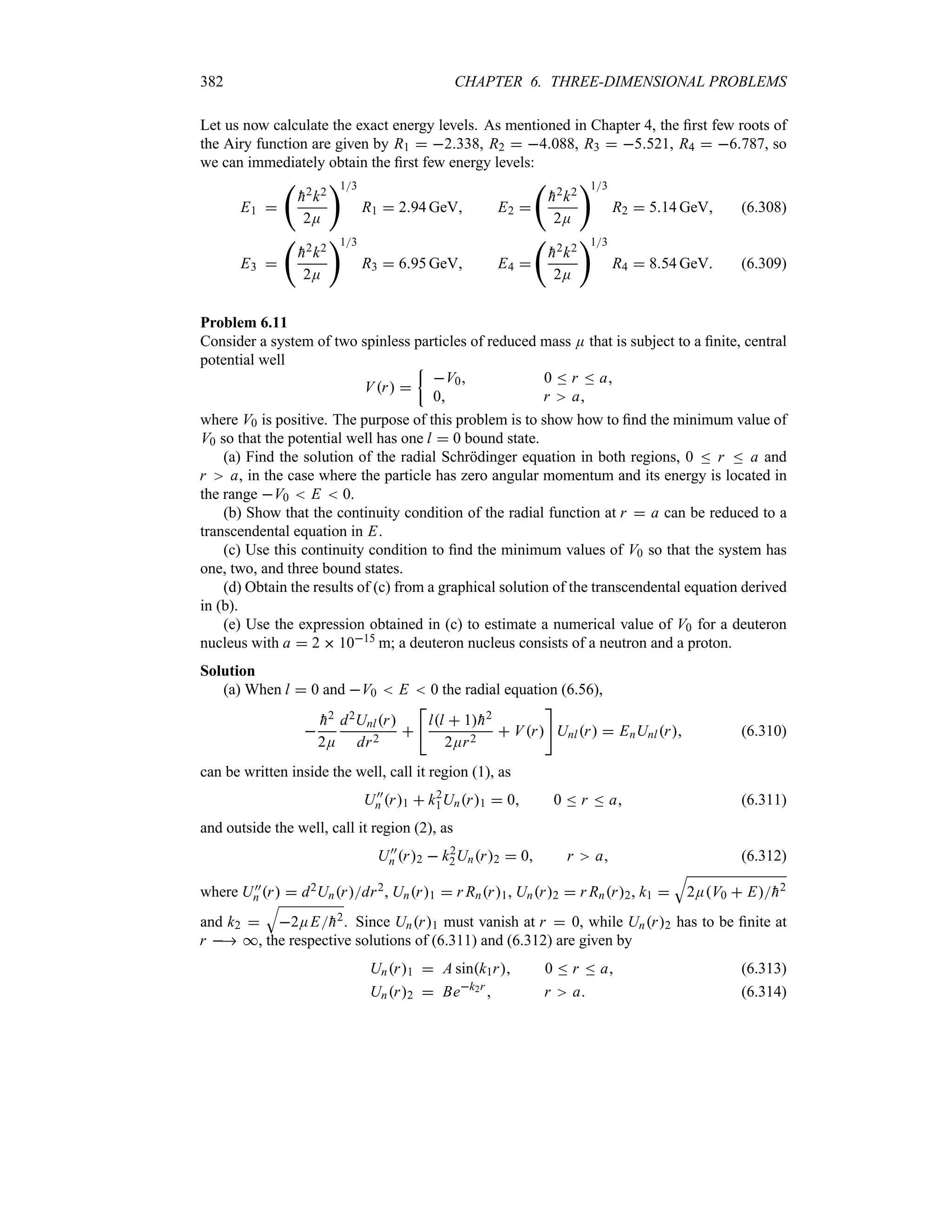
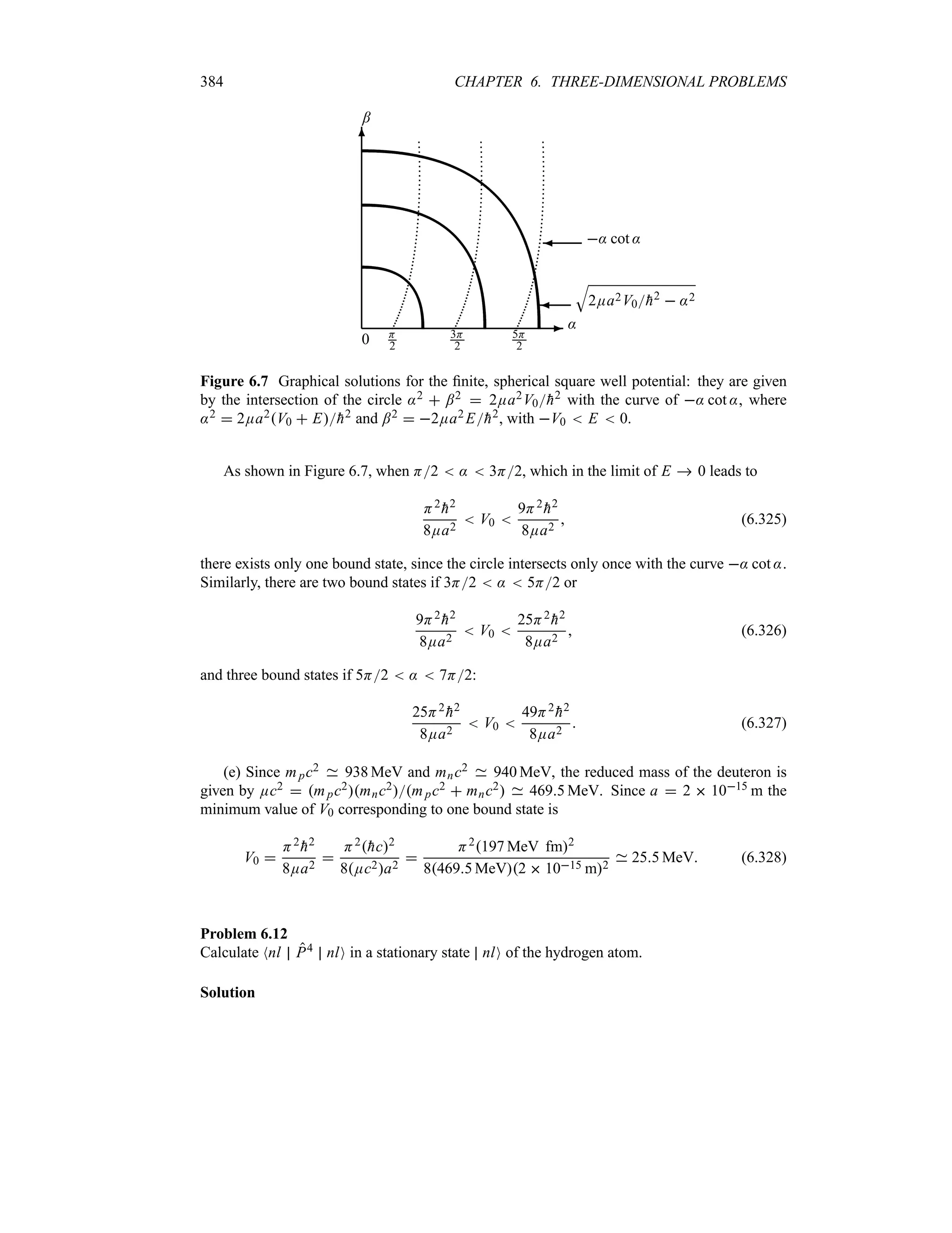
![6.6. EXERCISES 385
To calculate Nnl P4 nlO we may consider expressing P4 in terms of the hydrogen’s Hamil-
tonian. Since H P22me e2r we have P2 2meH e2r; hence
Nnl P4
nlO 2me2
nl
n
n
n
n
n
t
H
e2
r
u2
n
n
n
n
n
nl
2me2
~
nl
n
n
n
nH2
H
e2
r
e2
r
H
e4
r2
n
n
n
n nl
2me2
v
E2
n En
~
nl
n
n
n
n
e2
r
n
n
n
n nl
~
nl
n
n
n
n
e2
r
n
n
n
n nl
En
~
nl
n
n
n
n
e4
r2
n
n
n
n nl
w
(6.329)
where we have used the fact that nlO is an eigenstate of H: H nlO En nlO with
En e22a0n2 136 eVn2. The expectation values of 1r and 1r2 are given by
(6.182) and (6.183), Nnl r1 nlO 1n2a0 and Nnl r2 nlO 2[n32l 1a2
0]; we can thus
rewrite (6.329) as
Nnl P4
nlO 2me2
v
E2
n 2En
~
nl
n
n
n
n
e2
r
n
n
n
n nl
~
nl
n
n
n
n
e4
r2
n
n
n
n nl
w
2me En2
1
2e2
En
1
n2 a0
e4
E2
n
2
n32l 1a2
0
2me En2
v
1 4
8n
2l 1
w
(6.330)
in deriving the last relation we have used En e22a0n2. Now, since a0
h2mee2, the
energy En becomes En e22a0n2 mee42
h2n2 which, when inserted into (6.330),
leads to
Nnl P4
nlO
m4
ee8
h4n4
v
8n
2l 1
3
w
(6.331)
6.6 Exercises
Exercise 6.1
A spinless particle of mass m is confined to move in the xy plane under the influence of a
harmonic oscillator potential Vx y 1
2 m2
b
x2 y2
c
for all values of x and y.
(a) Show that the Hamiltonian H of this particle can be written as a sum of two familiar one-
dimensional Hamiltonians, Hx and Hy. Then show that H commutes with Lz X Py Y Px.
(b) Find the expression for the energy levels Enx ny .
(c) Find the energies of the four lowest states and their corresponding degeneracies.
(d) Find the degeneracy gn of the nth excited state as a function of the quantum number n
(n nx ny).
(e) If the state vector of the nth excited state is nO nxO nyO or
Nxy nO Nx nxONy nyO Onx xOny y](https://image.slidesharecdn.com/zettili-250217213640-909f6141/75/Zettili-Quantum-mechanics-Concept-and-application-pdf-402-2048.jpg)
![386 CHAPTER 6. THREE-DIMENSIONAL PROBLEMS
calculate the expectation value of the operator A x4 y2 in the state nO as a function of the
quantum numbers nx and ny.
Exercise 6.2
A particle of mass m moves in the xy plane in the potential
Vx y
| 1
2 m2 y2 for all y and 0 x a
* elsewhere
(a) Write down the time-independent Schrödinger equation for this particle and reduce it to
a set of familiar one-dimensional equations.
(b) Find the normalized eigenfunctions and the eigenenergies.
Exercise 6.3
A particle of mass m moves in the xy plane in a two-dimensional rectangular well
Vx y
|
0 0 x a 0 y b
* elsewhere
By reducing the time-independent Schrödinger equation to a set of more familiar one-dimensional
equations, find the normalized wave functions and the energy levels of this particle.
Exercise 6.4
Consider an anisotropic three-dimensional harmonic oscillator potential
Vx y z
1
2
m2
x x2
2
y y2
2
z z2
(a) Evaluate the energy levels in terms of x , y, and z.
(b) Calculate [H Lz]. Do you expect the wave functions to be eigenfunctions of ;
L2?
(c) Find the three lowest levels for the case x y 2z3, and determine the degener-
acy of each level.
Exercise 6.5
Consider a spinless particle of mass m which is confined to move under the influence of a
three-dimensional potential
Vx y z
|
0 for 0 x a 0 y a 0 z b
* elsewhere
(a) Find the expression for the energy levels Enx nynz and their corresponding wave func-
tions.
(b) If a 2b find the energies of the five lowest states and their degeneracies.
Exercise 6.6
A particle of mass m moves in the three-dimensional potential
Vx y z
| 1
2 m2z2 for 0 x a 0 y a and z 0
* elsewhere](https://image.slidesharecdn.com/zettili-250217213640-909f6141/75/Zettili-Quantum-mechanics-Concept-and-application-pdf-403-2048.jpg)
![390 CHAPTER 6. THREE-DIMENSIONAL PROBLEMS
Exercise 6.20
The wave function of a hydrogen-like atom at time t 0 is
;
r 0
1
T
11
KT
3O211;
r O210;
r
T
5O211;
r
T
2O311;
r
L
where Onlm;
r is a normalized eigenfunction (i.e., Onlm;
r RnlrYlmA ).
(a) What is the time-dependent wave function?
(b) If a measurement of energy is made, what values could be found and with what proba-
bilities?
(c) What is the probability for a measurement of Lz which yields 1
h?
Exercise 6.21
Using the fact that the radial momentum operator is given by pr i
h 1
r
r r, calculate the
commutator [r pr ] between the position operator, r, and the radial momentum operator.
Exercise 6.22
Calculate rpr with respect to the state
O210;
r
1
T
6
t
1
a0
u32
r
2a0
er2a0 Y10A
and verify that rpr satisfies the Heisenberg uncertainty principle.](https://image.slidesharecdn.com/zettili-250217213640-909f6141/75/Zettili-Quantum-mechanics-Concept-and-application-pdf-407-2048.jpg)
![394 CHAPTER 7. ROTATIONS AND ADDITION OF ANGULAR MOMENTA
We may generalize this relation to a rotation of angle =M about an arbitrary axis whose direction
is given by the unit vector ;
n:
R=M 1
i
h
=M ;
n ;
L (7.21)
This is the operator corresponding to an infinitesimal rotation of angle =M about ;
n for a spinless
system. The orbital angular momentum is thus the generator of infinitesimal spatial rotations.
Rotations and the commutation relations
We can show that the relation (7.10) leads to the commutation relations of angular momentum
[Lx Ly] i
hLz. The operators corresponding to infinitesimal rotations of angle = about the
x and y axes can be inferred from (7.20):
Rx = 1
i=
h
Lx
=2
2
h2
L2
x Ry= 1
i=
h
Ly
=2
2
h2
L2
y (7.22)
where we have extended the expansions to the second power in =. On the one hand, the follow-
ing useful relation can be obtained from (7.22):
Rx=Ry= Ry=Rx=
t
1
i=
h
Lx
=2
2
h2
L2
x
u t
1
i=
h
Ly
=2
2
h2
L2
y
u
t
1
i=
h
Ly
=2
2
h2
L2
y
u t
1
i=
h
Lx
=2
2
h2
L2
x
u
=2
h2
r
Lx Ly Ly Lx
s
=2
h2
[Lx Ly] (7.23)
where we have kept only terms up to the second power in =; the terms in = cancel out automat-
ically.
On the other hand, according to (7.10), we have
Rx=Ry= Ry=Rx= Rz=2
1 (7.24)
Since Rz=2 1 i=2
hLz this relations leads to
Rx=Ry= Ry=Rx= Rz=2
1
i=2
h
Lz (7.25)
Finally, equating (7.23) and (7.25), we end up with
[Lx Ly] i
hLz (7.26)
Similar calculations for Ry=Rz= Rz=Ry= and Rz=Rx = Rx=Rz= lead to the
other two commutation relations [Ly Lz] i
hLx and [Lz Lx] i
hLy.](https://image.slidesharecdn.com/zettili-250217213640-909f6141/75/Zettili-Quantum-mechanics-Concept-and-application-pdf-411-2048.jpg)
![7.2. ROTATIONS IN QUANTUM MECHANICS 395
7.2.2 Finite Rotations
The operator RzM corresponding to a rotation (of the coordinates of a spinless particle) over a
finite angle M about the z-axis can be constructed in terms of the infinitesimal rotation operator
(7.20) as follows. We divide the angle M into N infinitesimal angles =M: M N =M. The
rotation over the finite angle M can thus be viewed as a series of N consecutive infinitesimal
rotations, each over the angle =M, about the z-axis, applied consecutively one after the other:
RzM RzN=M Rz=MN
t
1 i
=M
h
Lz
uN
(7.27)
Since =M MN, and if =M is infinitesimally small, we have
RzM lim
N*
N
k1
t
1
i
h
M
N
n ;
L
u
lim
N*
t
1
i
h
M
N
Lz
uN
(7.28)
or
RzM eiMLz
h
(7.29)
We can generalize this result to infer the rotation operator RnM corresponding to a rotation
over a finite angle M around an axis ;
n:
RnM eiM;
n;
L
h
(7.30)
where ;
L is the orbital angular momentum. This operator represents the rotation of the coordi-
nates of a spinless particle over an angle M about an axis ;
n.
The discussion that led to (7.30) was carried out for a spinless system. A more general
study for a system with spin would lead to a relation similar to (7.30):
RnM e i
h M;
n ;
J
(7.31)
where ;
J is the total angular momentum operator; this is known as the rotation operator. For
instance, the rotation operator ;
RxM of a rotation through an angle M about the x-axis is given
by
Rx M eiMJx
h
(7.32)
The properties of RnM are determined by those of the operators Jx Jy Jz.
Remark
The Hamiltonian of a particle in a central potential, H P22m Vr, is invariant under
spatial rotations since, as shown in Chapter 6, it commutes with the orbital angular momentum:
[H ;
L] 0
v
H eiM;
n;
L
h
w
0 (7.33)
Due to this symmetry of space isotropy or rotational invariance, the orbital angular momentum
is conserved1. So, in the case of particles moving in central potentials, the orbital angular
momentum is a constant of the motion.
1In classical physics when a system is invariant under rotations, its total angular momentum is also conserved.](https://image.slidesharecdn.com/zettili-250217213640-909f6141/75/Zettili-Quantum-mechanics-Concept-and-application-pdf-412-2048.jpg)
![396 CHAPTER 7. ROTATIONS AND ADDITION OF ANGULAR MOMENTA
7.2.3 Properties of the Rotation Operator
The rotation operators constitute a representation of the rotation group and satisfy the following
properties:
The product of any two rotation operators is another rotation operator:
Rn1 Rn2 Rn3 (7.34)
The associative law holds for rotation operators:
r
Rn1 Rn2
s
Rn3 Rn1
r
Rn2 Rn3
s
(7.35)
The identity operator (corresponding to no rotation) satisfies the relation
I Rn Rn I Rn (7.36)
From (7.31) we see that for each rotation operator Rn, there exists an inverse operator
R1
n so that
Rn R1
n R1
n Rn I (7.37)
The operator Rn, which is equal to R1
n , corresponds to a rotation in the opposite sense
to Rn.
In sharp contrast to the translation group2 in three dimensions, the rotation group is not com-
mutative (nonabelian). The product of two rotation operators depends on the order in which
they are performed:
Rn1 MRn2 A / Rn2 ARn1 M (7.38)
this is due to the fact that the commutator [;
n1 ;
J ;
n2 ;
J] is not zero. In this way, the rotation
group is in general nonabelian.
But if the two rotations were performed about the same axis, the corresponding operators
would commute:
RnMRnA RnARnM RnM A (7.39)
Note that, since the angular momentum operator J is Hermitian, equation (7.31) yields
R
†
n M R1
n M RnM eiM;
n ;
J
h
(7.40)
hence the rotation operator (7.31) is unitary:
R
†
n M R1
n M R
†
n MRnM I (7.41)
The operator RnM therefore conserves the scalar product of kets, notably the norm of vectors.
For instance, using
O)
O RnM OO N)
O RnM NO (7.42)
along with (7.41), we can show that NN) O)O NN OO, since
NN)
O)
O NN R
†
n MRnM OO NN OO (7.43)
2The linear momenta Pi and Pj —which are the generators of translation—commute even when i / j; hence the
translation group is said to be abelian.](https://image.slidesharecdn.com/zettili-250217213640-909f6141/75/Zettili-Quantum-mechanics-Concept-and-application-pdf-413-2048.jpg)
![398 CHAPTER 7. ROTATIONS AND ADDITION OF ANGULAR MOMENTA
The inverse transformation of (7.48) is obtained by taking three rotations in reverse order over
the angles ; ::
R1
: ; Rz Ry;Rz: R†: ; ei Jz
h
ei; Jy
h
ei:Jz
h
(7.49)
7.2.5 Representation of the Rotation Operator
The rotation operator R: ; as given by (7.48) implies that its properties are determined
by the algebraic properties of the angular momentum operators Jx, Jy, Jz. Since R: ;
commutes with ;
J2, we may look for a representation of R: ; in the basis spanned by the
eigenvectors of ;
J2 and Jz, i.e., the j mO states.
From (7.48), we see that;
J2 commutes with the rotation operator, [ ;
J2 R: ; ] 0;
thus, the total angular momentum is conserved under rotations
;
J2
R: ; j mO R: ; ;
J2
j mO j j 1R: ; j mO (7.50)
However, the z-component of the angular momentum changes under rotations, unless the axis
of rotation is along the z-axis. That is, when R: ; acts on the state j mO, we end up
with a new state having the same j but with a different value of m:
R: ; j mO
j
;
m) j
j m)
ON j m)
R: ; j mO
j
;
m) j
D
j
m)m: ; j m)
O (7.51)
where
D
j
m)m: ; N j m)
R: ; j mO (7.52)
These are the matrix elements of R: ; for the j mO states; D
j
m)m: ; is the am-
plitude of j m)O when j mO is rotated. The rotation operator is thus represented by a
2 j 1 2 j 1 square matrix in the j mO basis. The matrix of D j: ; is known
as the Wigner D-matrix and its elements D
j
m)m: ; as the Wigner functions. This matrix
representation is often referred to as the 2 j 1-dimensional irreducible representation of the
rotation operator R: ; .
Since j mO is an eigenstate of Jz, it is also an eigenstate of the rotation operator ei:Jz
h,
because
ei:Jz
h
j mO ei:m
j mO (7.53)
We may thus rewrite (7.52) as
D
j
m)m: ; eim):m
d
j
m)m; (7.54)
where
d
j
m)m; N j m)
ei; Jy
h
j mO (7.55)](https://image.slidesharecdn.com/zettili-250217213640-909f6141/75/Zettili-Quantum-mechanics-Concept-and-application-pdf-415-2048.jpg)


![408 CHAPTER 7. ROTATIONS AND ADDITION OF ANGULAR MOMENTA
Thus, for every j the allowed values of m are located within the range j n m n j.
Note that the coefficient N j1 j2 m1 m2 j mO vanishes unless m1 m2 m. This can
be seen as follows: since Jz J1z J2z , we have
N j1 j2 m1 m2 Jz J1z J2z j mO 0 (7.132)
and since Jz j mO m
h j mO, N j1 j2 m1 m2 J1z m1
hN j1 j2 m1 m2 , and
N j1 j2 m1 m2 J2z m2
hN j1 j2 m1 m2 we can write
m m1 m2 N j1 j2 m1 m2 j mO 0 (7.133)
which shows that N j1 j2 m1 m2 j mO is not zero only when m m1 m2 0.
If m1 m2 / m N j1 j2 m1 m2 j mO 0 (7.134)
So, for the Clebsch–Gordan coefficient N j1 j2 m1 m2 j mO not to be zero, we must simul-
taneously have
m1 m2 m and j1 j2 n j n j1 j2 (7.135)
These are known as the selection rules for the Clebsch–Gordan coefficients.
Example 7.2
Starting from
3jmax
j jmin
2 j 1 2 j1 12 j2 1, prove (7.129).
Solution
Let us first work on the left-hand side of
jmax
;
j jmin
2 j 1 2 j1 1 2 j2 1 (7.136)
Since jmax j1 j2 we can write the left-hand side of this equation as an arithmetic sum
which has jmax jmin 1 [ j1 j2 1 jmin] terms:
jmax
;
j jmin
2 j 1 2 jmin 12 jmin 32 jmin 5
d
2 j1 j2 1
e
(7.137)
To calculate this sum, we simply write it in the following two equivalent ways:
S 2 jmin 1 2 jmin 3 2 jmin 5 [2 j1 j2 1] (7.138)
S [2 j1 j2 1] [2 j1 j2 1] [2 j1 j2 3] 2 jmin 1 (7.139)
Adding these two series term by term, we obtain
2S 2[ j1 j2 1 jmin]2[ j1 j2 1 jmin] 2[ j1 j2 1 jmin] (7.140)
Since this expression has jmax jmin 1 [ j1 j2 1 jmin] terms, we have
2S 2[ j1 j2 1 jmin][ j1 j2 1 jmin] (7.141)](https://image.slidesharecdn.com/zettili-250217213640-909f6141/75/Zettili-Quantum-mechanics-Concept-and-application-pdf-425-2048.jpg)
![7.3. ADDITION OF ANGULAR MOMENTA 409
hence
S [ j1 j2 1 jmin][ j1 j2 1 jmin] j1 j2 12
j2
min (7.142)
Now, equating this expression with the right-hand side of (7.136), we obtain
j1 j2 12
j2
min 2 j1 1 2 j2 1 (7.143)
which in turn leads to
j2
min j1 j22
(7.144)
7.3.2 Calculation of the Clebsch–Gordan Coefficients
First, we should point out that the Clebsch–Gordan coefficients corresponding to the two lim-
iting cases where m1 j1, m2 j2, j j1 j2, m j1 j2 and m1 j1, m2 j2,
j j1 j2, m j1 j2 are equal to one:
N j1 j2 j1 j2 j1 j2 j1 j2O 1 N j1 j2 j1 j2 j1 j2 j1 j2O 1
(7.145)
These results can be inferred from (7.121), since j1 j2 j1 j2O, and j1 j2 j1 j2O
have one element each:
j1 j2 j1 j2O N j1 j2 j1 j2 j1 j2 j1 j2O j1 j2 j1 j2O (7.146)
j1 j2 j1 j2O N j1 j2 j1 j2 j1 j2 j1 j2O j1 j2 j1 j2O (7.147)
where j1 j2 j1 j2O, j1 j2 j1 j2O, j1 j2 j1 j2O, and j1 j2 j1 j2O
are all normalized.
The calculations of the other coefficients are generally more involved than the two limiting
cases mentioned above. For this, we need to derive the recursion relations between the matrix
elements of the unitary transformation between the j mO and j1 j2 m1 m2O bases,
since, when j1, j2 and j are fixed, the various Clebsch–Gordan coefficients are related to one
another by means of recursion relations. To find the recursion relations, we need to evaluate the
matrix elements N j1 j2 m1 m2 J j mO in two different ways. First, allow J to act to
the right, i.e., on j mO:
N j1 j2 m1 m2 J j mO
h
S
j b m j m 1N j1 j2 m1 m2 j m 1O (7.148)
Second, make J J1 J2 act to the left6, i.e., on N j1 j2 m1 m2 :
N j1 j2 m1 m2 J j mO
h
S
j1 m1 j1 b m1 1N j1 j2 m1 b 1 m2 j mO
h
S
j2 m2 j2 b m2 1N j1 j2 m1 m2 b 1 j mO (7.149)
6Recall that N j1 j2 m1 m2 J1
h
T
j1 m1 j1 b m1 1N j1 j2 m1 b 1 m2 .](https://image.slidesharecdn.com/zettili-250217213640-909f6141/75/Zettili-Quantum-mechanics-Concept-and-application-pdf-426-2048.jpg)
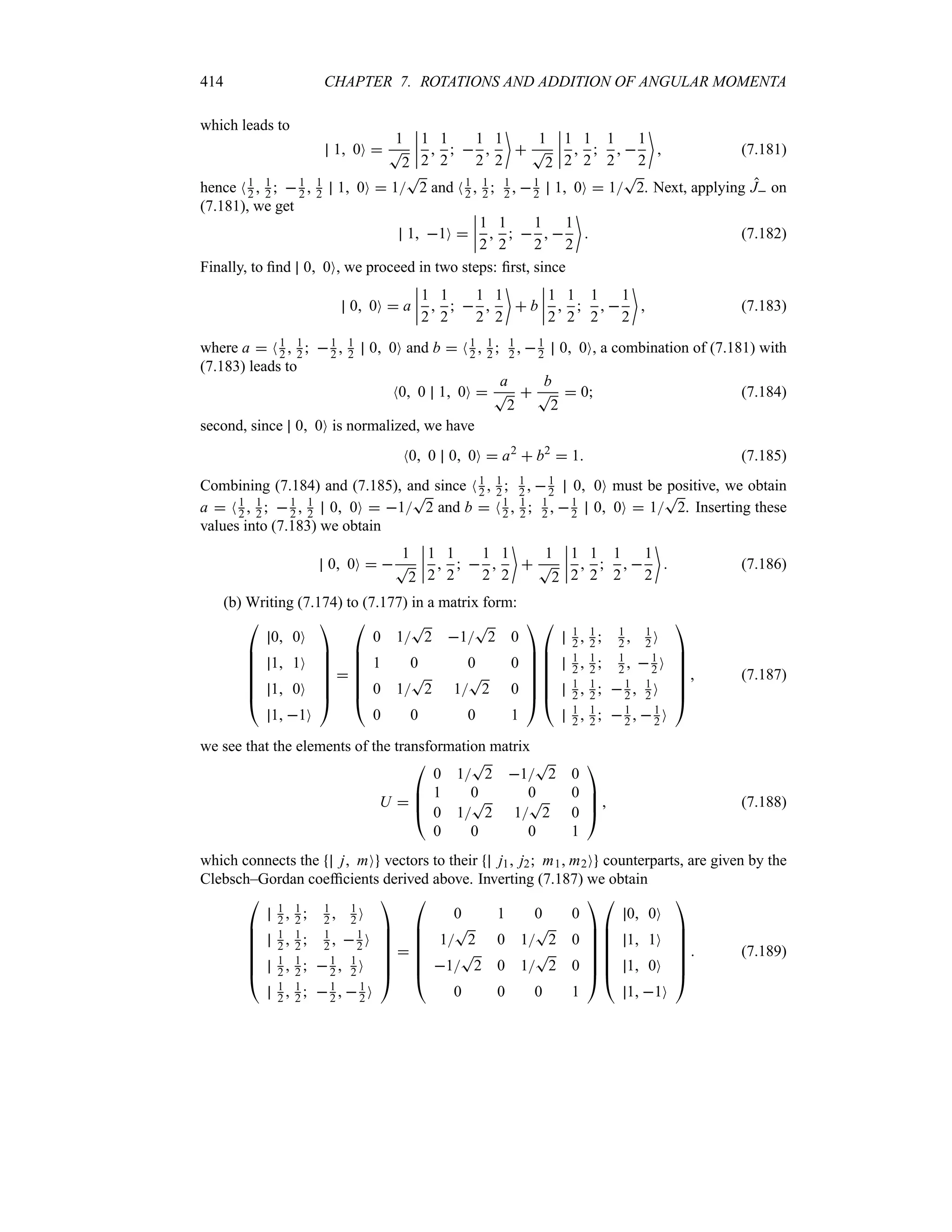
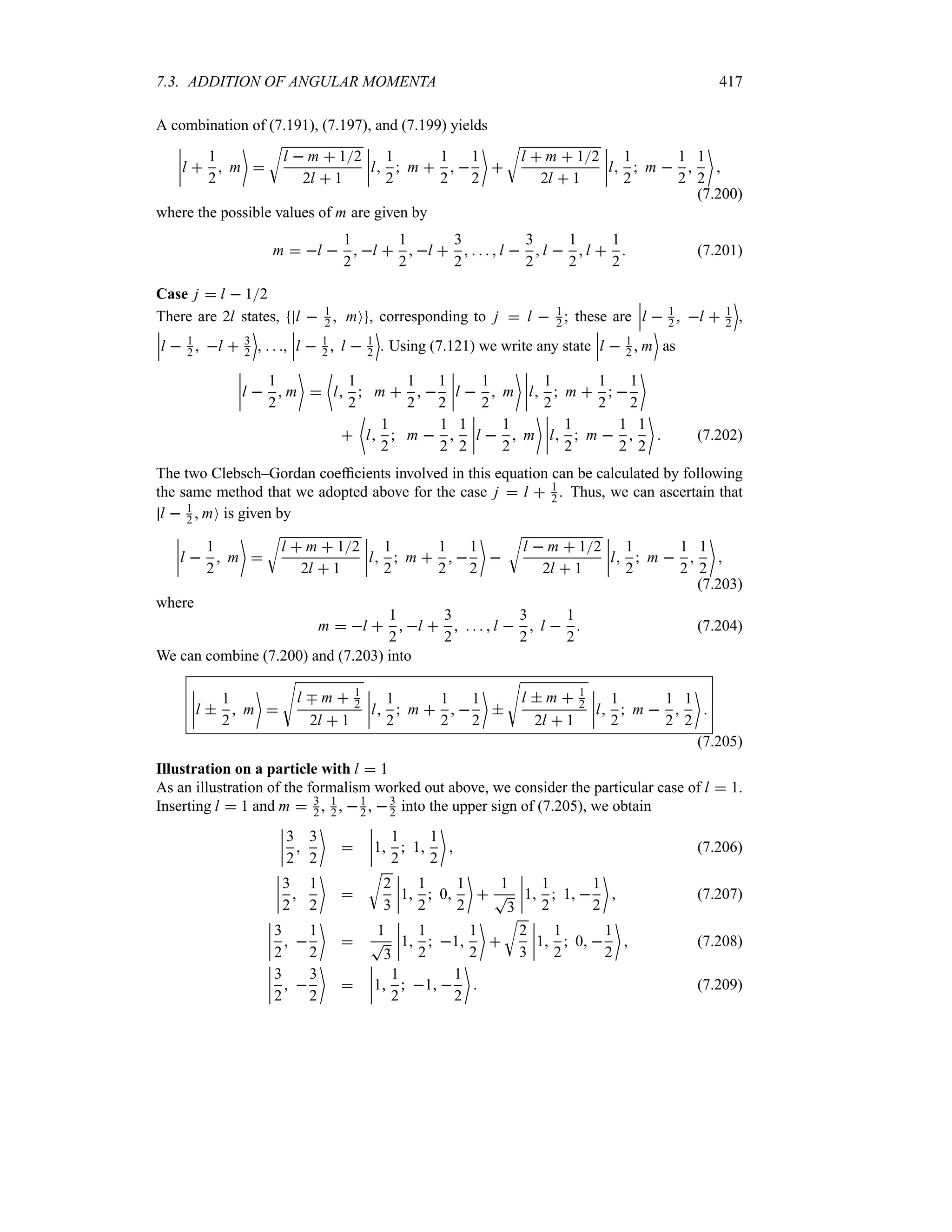
![420 CHAPTER 7. ROTATIONS AND ADDITION OF ANGULAR MOMENTA
the problem to the coupling of N 1 angular momenta. For instance, we may start by adding
;
J1 and ;
J2 to generate ;
J12; we are then left with N 1 angular momenta. Second, by adding
;
J12 and ;
J3 to form ;
J123, we are left with N 2 angular momenta. Third, an addition of ;
J123
and ;
J4 leaves us with N 3 angular momenta, and so on. We may continue in this way till
we add all given angular momenta.
7.3.5 Rotation Matrices for Coupling Two Angular Momenta
We want to find out how to express the rotation matrix associated with an angular momentum
;
J in terms of the rotation matrices corresponding to ;
J1 and ;
J2 such that ;
J ;
J1 ;
J2. That is,
knowing the rotation matrices d j1; and d j2;, how does one calculate d
j
mm) ;?
Since
d
j
m)m; N j m)
Ry; j mO (7.224)
where
j mO
;
m1m2
N j1 j2 m1 m2 j mO j1 j2 m1 m2O (7.225)
j m)
O
;
m)
1m)
2
N j1 j2 m)
1 m)
2 j m)
O j1 j2 m)
1 m)
2O (7.226)
and since the Clebsch–Gordan coefficients are real,
N j m)
;
m)
1m)
2
N j1 j2 m)
1 m)
2 j m)
ON j1 j2 m)
1 m)
2 (7.227)
we can rewrite (7.224) as
d
j
m)m;
;
m1m2
;
m)
1m)
2
N j1 j2 m1 m2 j mON j1 j2 m)
1 m)
2 j m)
O
N j1 j2 m)
1 m)
2 Ry; j1 j2 m1 m2O (7.228)
Since Ry; exp[; Jy
h] exp[; J1y
h] exp[; J2y
h], because Jy J1y J2y , and
since N j1 j2 m)
1 m)
2 N j1 m)
1 N j2 m)
2 and j1 j2 m1 m2O j1 m1O j2 m2O, we
have
d
j
m)m;
;
m1m2
;
m)
1m)
2
N j1 j2 m1 m2 j mON j1 j2 m)
1 m)
2 j m)
O
N j1 m)
1 exp
v
i
h
; J1y
w
j1 m1ON j2 m)
2 exp
v
i
h
; J2y
w
j2 m2O
(7.229)
or
d
j
m)m;
;
m1m2
;
m)
1m)
2
N j1 j2 m1 m2 j mON j1 j2 m)
1 m)
2 j m)
Od
j1
m)
1m1
;d
j2
m)
2m2
;
(7.230)](https://image.slidesharecdn.com/zettili-250217213640-909f6141/75/Zettili-Quantum-mechanics-Concept-and-application-pdf-437-2048.jpg)


![426 CHAPTER 7. ROTATIONS AND ADDITION OF ANGULAR MOMENTA
where Rn=A can be inferred from (7.20)
Rn=A 1
i
h
=A ;
n ;
J (7.275)
Substituting (7.275) into (7.274) and keeping terms up to first order in =A, we obtain
A)
A
i
h
=A [A ;
n ;
J ] (7.276)
In the rest of this section we focus on the application of this relation to scalar, vector, and tensor
operators.
7.4.1 Scalar Operators
Since scalar operators are invariant under rotations (i.e., A) A, equation (7.276) implies that
they commute with the angular momentum
[A Jk ] 0 k x y z (7.277)
This is also true for pseudo-scalars. A pseudo-scalar is defined by the product of a vector ;
A
and a pseudo-vector or axial vector ;
B ;
C: ;
A ;
B ;
C.
7.4.2 Vector Operators
On the one hand, a vector operator ;
A transforms according to (7.276):
;
A )
;
A
i
h
=A [ ;
A ;
n ;
J ] (7.278)
On the other hand, from the classical theory of rotations, when a vector ;
A is rotated through an
angle =A around an axis ;
n, it is given by
;
A )
;
A =A ;
n ;
A (7.279)
Comparing (7.278) and (7.279), we obtain
[ ;
A ;
n ;
J ] i
h;
n ;
A (7.280)
The jth component of this equation is given by
[ ;
A ;
n ;
J ]j i
h;
n ;
Aj j x y z (7.281)
which in the case of j x y z leads to
K
Ax Jx
L
K
Ay Jy
L
K
Az Jz
L
0 (7.282)
K
Ax Jy
L
i
hAz
K
Ay Jz
L
i
hAx
K
Az Jx
L
i
hAy (7.283)
K
Ax Jz
L
i
hAy
K
Ay Jx
L
i
hAz
K
Az Jy
L
i
h Ax (7.284)](https://image.slidesharecdn.com/zettili-250217213640-909f6141/75/Zettili-Quantum-mechanics-Concept-and-application-pdf-443-2048.jpg)
![7.4. SCALAR, VECTOR, AND TENSOR OPERATORS 427
Some interesting applications of (7.280) correspond to the cases where the vector operator ;
A
is either the angular momentum, the position, or the linear momentum operator. Let us consider
these three cases separately. First, substituting ;
A ;
J into (7.280), we recover the usual angular
momentum commutation relations:
[Jx Jy] i
hJz [Jy Jz] i
hJx [Jz Jx ] i
hJy (7.285)
Second, in the case of a spinless particle (i.e., ;
J ;
L), and if ;
A is equal to the position operator,
;
A ;
R, then (7.280) will yield the following relations:
K
x Lx
L
0
K
x Ly
L
i
hz
K
x Lz
L
i
hy (7.286)
K
y Ly
L
0
K
y Lz
L
i
hx
K
y Lx
L
i
hz (7.287)
K
z Lz
L
0
K
z Lx
L
i
hy
K
z Ly
L
i
hx (7.288)
Third, if ;
J ;
L and if ;
A is equal to the momentum operator, ;
A ;
P, then (7.280) will lead to
K
Px Lx
L
0
K
Px Ly
L
i
hPz
K
Px Lz
L
i
hPy (7.289)
K
Py Ly
L
0
K
Py Lz
L
i
hPx
K
Py Lx
L
i
hPz (7.290)
K
Pz Lz
L
0
K
Pz Lx
L
i
hPy
K
Pz Ly
L
i
hPx (7.291)
Now, introducing the operators
A Ax i Ay (7.292)
and using the relations (7.282) to (7.284), we can show that
K
Jx A
L
b
hAz
K
Jy A
L
i
hAz
K
Jz A
L
hA (7.293)
These relations in turn can be shown to lead to
K
J A
L
0
K
J Ab
L
2
hAz (7.294)
Let us introduce the spherical components A1, A0, A1 of the vector operator A; they are
defined in terms of the Cartesian coordinates Ax Ay Az as follows:
A1 b
1
T
2
Ax Ay A0 Az (7.295)
For the particular case where A is equal to the position vector R, we can express the components
Rq (where q 1 0 1),
R1 b
1
T
2
x y R0 z (7.296)](https://image.slidesharecdn.com/zettili-250217213640-909f6141/75/Zettili-Quantum-mechanics-Concept-and-application-pdf-444-2048.jpg)

![436 CHAPTER 7. ROTATIONS AND ADDITION OF ANGULAR MOMENTA
(b) From (7.347) we can write
ei:Jx
Jzei:Jx
cos : iJx sin :Jzcos : iJx sin :
Jz cos2
: Jx JzJx sin2
: i[Jx Jz] sin : cos :
(7.348)
which, when using the facts that JxJz JzJx , J2
x I, and [Jx Jz] 2iJy, reduces to
ei:Jx Jzei:Jx Jz cos2
: JzJ2
x sin2
: 2Jy sin : cos :
Jzcos2
: sin2
: Jy sin2:
Jz cos2: Jy sin2: (7.349)
Problem 7.3
Find the Clebsch–Gordan coefficients associated with the addition of two angular momenta
j1 1 and j2 1.
Solution
The addition of j1 1 and j2 1 is encountered, for example, in a two-particle system where
the angular momenta of both particles are orbital.
The allowed values of the total angular momentum are between j1 j2 n j n j1 j2;
hence j 0, 1, 2. To calculate the relevant Clebsch–Gordan coefficients, we need to find
the basis vectors j mO , which are common eigenvectors of ;
J2
1, ;
J2
2, ;
J2 and Jz, in terms of
1 1 m1 m2O .
Eigenvectors j mO associated with j 2
The state 2 2O is simply given by
2 2O 1 1 1 1O (7.350)
the corresponding Clebsch–Gordan coefficient is thus given by N1 1 1 1 2 2O 1.
As for 2 1O, it can be found by applying J to 2 2O and J1 J2 to 1 1 1 1O, and
then equating the two results
J 2 2O
b
J1 J2
c
1 1 1 1O (7.351)
This leads to
2
h 2 1O
T
2
h
r
1 1 1 0O 1 1 0 1O
s
(7.352)
or to
2 1O
1
T
2
r
1 1 1 0O 1 1 0 1O
s
(7.353)
hence N1 1 1 0 2 1O N1 1 0 1 2 1O 1
T
2. Using (7.353), we can find 2 0O by
applying J to 2 1O and J1 J2 to [ 1 1 1 0O 1 1 0 1O]:
J 2 1O
1
T
2
h
b
J1 J2
c
[ 1 1 1 0O 1 1 0 1O] (7.354)](https://image.slidesharecdn.com/zettili-250217213640-909f6141/75/Zettili-Quantum-mechanics-Concept-and-application-pdf-453-2048.jpg)
![7.5. SOLVED PROBLEMS 437
which leads to
2 0O
1
T
6
r
1 1 1 1O 2 1 1 0 0O 1 1 1 1O
s
(7.355)
hence N1 1 1 1 2 0O N1 1 1 1 2 0O 1
T
6 and N1 1 0 0 2 0O 2
T
6.
Similarly, by repeated applications of J and J1 J2 , we can show that
2 1O
1
T
2
r
1 1 0 1O 1 1 1 0O
s
(7.356)
2 2O 1 1 1 1O (7.357)
with N1 1 0 1 2 1O N1 1 1 0 2 1O 1
T
2 and N1 1 1 1 2 2O 1.
Eigenvectors j mO associated with j 1
The relation
1 mO
1
;
m11
1
;
m21
N1 1 m1 m2 1 mO 1 1 m1 m2O (7.358)
leads to
1 1O a 1 1 1 0O b 1 1 0 1O (7.359)
where a N1 1 1 0 1 1O and b N1 1 0 1 1 1O. Since 1 1O, 1 1 1 0O and
1 1 0 1O are all normalized, and since 1 1 1 0O is orthogonal to 1 1 0 1O and a and b
are real, we have
N1 1 1 1O a2
b2
1 (7.360)
Now, since N2 1 1 1O 0, equations (7.353) and (7.359) yield
N2 1 1 1O
a
T
2
b
T
2
0 (7.361)
A combination of (7.360) and (7.361) leads to a b 1
T
2. The signs of a and b have
yet to be found. The phase convention mandates that coefficients like N j1 j2 j1 j j1 j jO
must be positive. Thus, we have a 1
T
2 and b 1
T
2, which when inserted into (7.359)
give
1 1O
1
T
2
r
1 1 1 0O 1 1 0 1O
s
(7.362)
This yields N1 1 1 0 1 1O 1
2 and N1 1 0 1 1 1O 1
2 .
To find 1 0O we proceed as we did above when we obtained the states 2 1O, 2 0O, ,
2 2O by repeatedly applying J on 2 2O. In this way, the application of J on 1 1O and
b
J1 J2
c
on [ 1 1 1 0O 1 1 0 1O],
J 1 1O
1
2
b
J1 J2
c
[ 1 1 1 0O 1 1 0 1O] (7.363)
gives
T
2
h 1 0O
T
2
h
2
[ 1 1 1 1O 1 1 1 1O] (7.364)](https://image.slidesharecdn.com/zettili-250217213640-909f6141/75/Zettili-Quantum-mechanics-Concept-and-application-pdf-454-2048.jpg)
![7.5. SOLVED PROBLEMS 441
since ;
S12 ;
S3 1
2 [;
S12 ;
S32 S2
12 S2
3]. Since the operators H, S2, S2
12, and S2
3 mutually
commute, we may select as their joint eigenstates the kets s12 s mO; we have seen in (a) how
to construct these states. The eigenvalues of H are thus given by
H s12 s mO
0
2
h2
r
S2
S2
12 S2
3
s
s12 s mO
0
2
v
ss 1 s12s12 1
3
4
w
s12 s mO (7.386)
since s3 1
2 and S2
3 s12 s mO
h2s3s3 1 s12 s mO 3
h24 s12 s mO.
As shown in (7.386), the energy levels of this system are degenerate with respect to m, since
they depend on the quantum numbers s and s12 but not on m:
Es12s
0
2
v
ss 1 s12s12 1
3
4
w
(7.387)
For instance, the energy Es12s E132 02 is fourfold degenerate, since it corresponds
to four different states: s12 s mO 1 3
2 3
2 O and 1 3
2 1
2 O. Similarly, the energy
E012 0 is twofold degenerate; the corresponding states are 0 1
2 1
2 O. Finally, the energy
E112 0 is also twofold degenerate since it corresponds to 1 1
2 1
2 O.
Problem 7.5
Consider a system of four nonidentical spin 1
2 particles. Find the possible values of the total
spin S of this system and specify the number of angular momentum eigenstates, corresponding
to each value of S.
Solution
First, we need to couple two spins at a time: ;
S12 ;
S1 ;
S2 and ;
S34 ;
S3 ;
S4. Then we couple
;
S12 and ;
S34: ;
S ;
S12 ;
S34. From Problem 7.4, page 438, we have s12 0 1 and s34 0 1.
In total there are 16 states smO since 2s1 12s2 12s3 12s4 1 24 16.
Since s12 0 1 and s34 0 1, the coupling of ;
S12 and ;
S34 yields the following values for
the total spin s:
When s12 0 and s34 0 we have only one possible value, s 0, and hence only one
eigenstate, smO 0 0O.
When s12 1 and s34 0, we have s 1; there are three eigenstates: s mO 1 1O,
and 1 0O.
When s12 0 and s34 1, we have s 1; there are three eigenstates: smO 1 1O,
and 1 0O.
When s12 1 and s34 1 we have s 0 1 2; we have here nine eigenstates (see
Problem 7.3, page 436): 0 0O, 1 1O, 1 0O, 2 2O, 2 1O, and 2 0O.
In conclusion, the possible values of the total spin when coupling four 1
2 spins are s 0 1 2;
the value s 0 occurs twice, s 1 three times, and s 2 only once.](https://image.slidesharecdn.com/zettili-250217213640-909f6141/75/Zettili-Quantum-mechanics-Concept-and-application-pdf-458-2048.jpg)

![444 CHAPTER 7. ROTATIONS AND ADDITION OF ANGULAR MOMENTA
can be inferred from the triple integral relation (7.244):
Nl)
m)
Ykq l mO
V
2l 12k 1
4H2l) 1
Nl k 0 0 l)
0ONl k m q l)
m)
O (7.403)
We can then combine (7.401) and (7.403) to obtain the reduced matrix element
Nl)
P Yk
P lO
V
2l 12k 1
4H2l) 1
Nl k 0 0 l)
0O (7.404)
(b) To calculate Nn)l)m) ;
r nlmO it is more convenient to express the vector ;
r in terms of
the spherical components ;
r r1r0r1, which are given in terms of the Cartesian coordi-
nates x, y, z as follows:
r1
x iy
T
2
r
T
2
ei
sin A r0 z r cos A r1
x iy
T
2
r
T
2
ei
sin A
(7.405)
which in turn may be condensed into a single relation
rq
U
4H
3
rY1qA q 1 0 1 (7.406)
Next we may write Nn)l)m) rq nlmO in terms of a radial part and an angular part:
Nn)
l)
m)
rq nlmO
U
4H
3
Nn)
l)
rq nlONl)
m)
Y1qA l mO (7.407)
The calculation of the radial part, Nn)l) rq nlO
5 *
0 r3 R`
n)l) rR`
nlr dr, is straightforward
and is of no concern to us here; see Chapter 6 for its calculation. As for the angular part
Nl) m) Y1qA l mO, we can infer its expression from (7.403)
Nl)
m)
Y1q l mO
V
32l 1
4H2l) 1
Nl 1 0 0 l)
0ONl 1 m q l)
m)
O (7.408)
The Clebsch–Gordan coefficients Nl 1 m q l) m)O vanish unless m) m q and l 1 n
l) n l 1 or m m) m q 1 0 1 and l l) l 1 0 1. Notice that the case
l 0 is ruled out from the parity selection rule; so, the only permissible values of l) and l are
those for which l l) l 1. Obtaining the various relevant Clebsch–Gordan coefficients
from standard tables, we can ascertain that the only terms of (7.408) that survive are
Nl 1 m 1 Y11 l mO
V
3l m 1l m 2
8H2l 12l 3
(7.409)
Nl 1 m 1 Y11 l mO
V
3l m 1l m
8H2l 12l 3
(7.410)
Nl 1 m Y10 l mO
V
3[l 12 m2]
4H2l 12l 3
(7.411)](https://image.slidesharecdn.com/zettili-250217213640-909f6141/75/Zettili-Quantum-mechanics-Concept-and-application-pdf-461-2048.jpg)

![446 CHAPTER 7. ROTATIONS AND ADDITION OF ANGULAR MOMENTA
I
‚
Jy
h
2
*
;
n0
1n
2n!
;2n
1
i
Jy
h
*
;
n0
1n
2n 1!
;2n1
(7.419)
where I is the 3 3 unit matrix. Using the relations
3*
n0[1n2n!];2n cos ; and
3*
n0[1n2n 1!];2n1 sin ;, we may write
ei; Jy
h
I
‚
Jy
h
2
[cos ; 1] i
Jy
h
sin ; (7.420)
Inserting now the matrix expressions for Jy and J2
y as listed in (7.415) and (7.416), we obtain
ei; Jy
h
I
1
2
#
1 0 1
0 2 0
1 0 1
$ cos ; 1 i
i
T
2
#
0 1 0
1 0 1
0 1 0
$ sin ; (7.421)
or
d1
;
%
%
%
#
d1
11 d1
10 d1
11
d1
01 d1
00 d1
01
d1
11 d1
10 d1
11
$
%
%
%
#
1
2 1 cos ; 1
T
2
sin ; 1
2 1 cos ;
1
T
2
sin ; cos ; 1
T
2
sin ;
1
2 1 cos ; 1
T
2
sin ; 1
2 1 cos ;
$
(7.422)
Since 1
2 1 cos ; cos2;2 and 1
2 1 cos ; sin2
;2, we have
d1
; ei; Jy
h
%
%
%
#
cos2;2 1
T
2
sin; sin2
;2
1
T
2
sin; cos; 1
T
2
sin;
sin2
;2 1
T
2
sin; cos2;2
$
(7.423)
This method becomes quite intractable when attempting to derive the matrix of d j; for
large values of j. In Problem 7.10 we are going to present a simpler method for deriving d j;
for larger values of j; this method is based on the addition of angular momenta.
Problem 7.10
(a) Use the relation
d
j
mm) ;
;
m1m2
;
m)
1m)
2
N j1 j2 m1 m2 j mON j1 j2 m)
1 m)
2 j m)
O d
j1
m1m)
1
;d
j2
m2m)
2
;
for the case where j1 1 and j2 1
2 along with the Clebsch–Gordan coefficients derived in
(7.206) to (7.209), and the matrix elements of d12; and d1;, which are given by (7.89)
and (7.423), respectively, to find the expressions of the matrix elements of d
32
3
2
3
2
;, d
32
3
2
1
2
;,
d
32
3
2 1
2
;, d
32
3
2 3
2
;, d
32
1
2
1
2
;, and d
32
1
2 1
2
;.
(b) Use the six expressions derived in (a) to infer the matrix of d32;.](https://image.slidesharecdn.com/zettili-250217213640-909f6141/75/Zettili-Quantum-mechanics-Concept-and-application-pdf-463-2048.jpg)
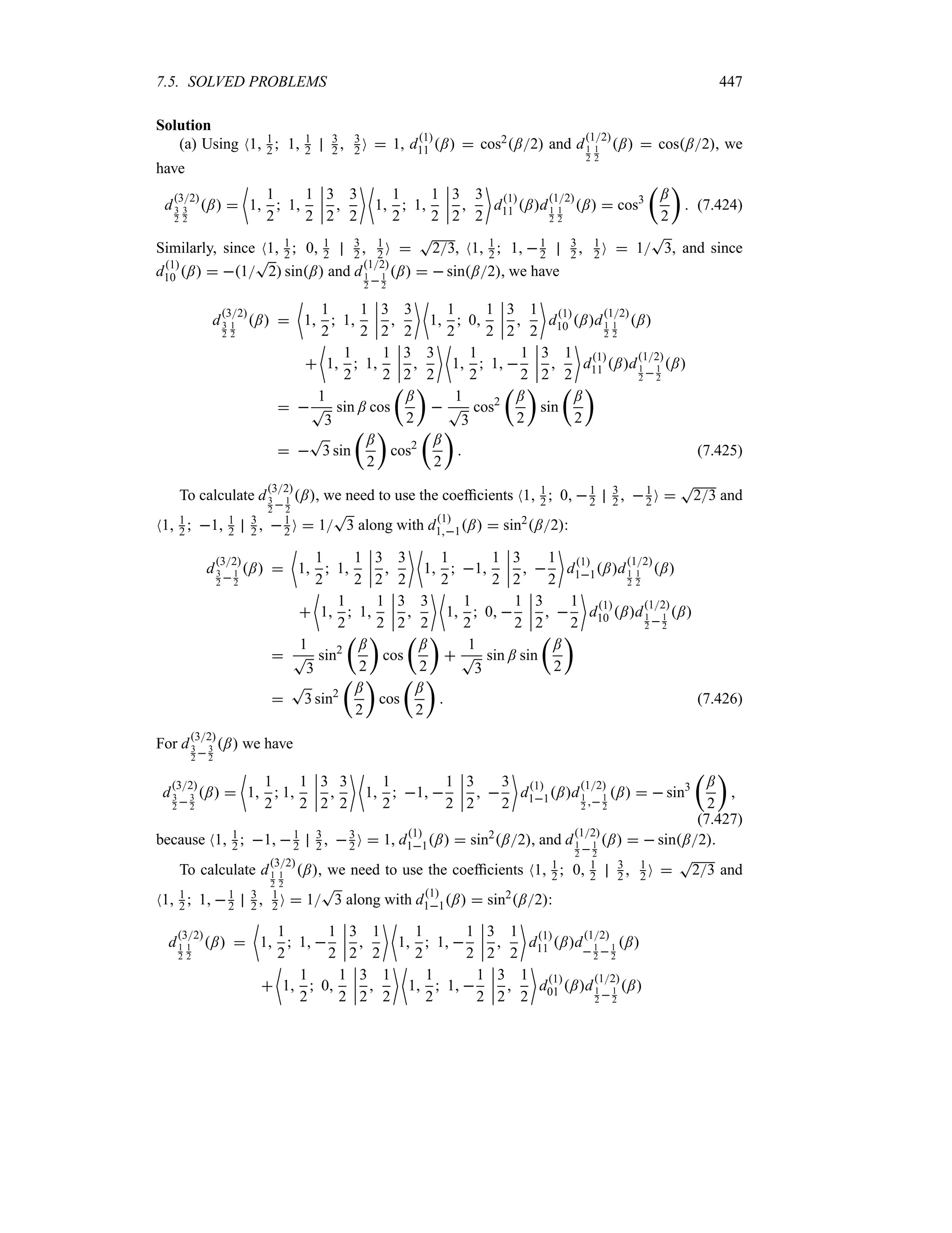
![7.6. EXERCISES 453
Exercise 7.20
Calculate the trace of the rotation matrix D12: ; for (a) ; H and (b) : H and
; 2H.
Exercise 7.21
The quadrupole moment operator of a charge q is given by Q20 q3z2 r2. Write Q20 in
terms of an irreducible spherical tensor of rank 2 and then express N j j Q20 j jO in terms
of j and the reduced matrix element N j P r2Y2 P jO. Hint: You may use the coefficient
N j 2 m 0 j mO 1jm[3m2 j j 1]
T
2 j 1 j j 12 j 3.
Exercise 7.22
Prove the following commutation relations:
(a)
K
Jx [Jx Tk
q ]
L
3
q) T k
q) Nk q) J2
x k qO,
(b)
K
Jx [Jx Tk
q ]
L
K
Jy [Jy Tk
q ]
L
K
Jz [Jz Tk
q ]
L
kk 1
h2T k
q .
Exercise 7.23
Consider a spin 1
2 particle which has an orbital angular momentum l 1. Find all the Clebsch–
Gordan coefficients involved in the addition of the orbital and spin angular momenta of this
particle. Hint: The Clebsch–Gordan coefficient N j1 j2 j1 j2 j1 j2 j2O is real and
positive.
Exercise 7.24
This problem deals with another derivation of the matrix elements of d1;. Use the relation
d
j
mm) ;
;
m1m2
;
m)
1m)
2
N j1 j2 m1 m2 j mON j1 j2 m)
1 m)
2 j m)
O d
j1
m1m)
1
;d
j2
m2m)
2
;
for the case where j1 j2 1
2 along with the matrix elements of d12;, which are given
by (7.89), to derive all the matrix elements of d1;.
Exercise 7.25
Consider the tensor AA sin2
A cos2 .
(a) Calculate the reduced matrix element N2 P Y2 P 2O. Hint: You may calculate explicitly
N2 1 Y20 2 1O and then use the Wigner–Eckart theorem to calculate it again.
(b) Express AA in terms of the components of a spherical tensor of rank 2 (i.e., in terms
of Y2mA ).
(c) Calculate Am)1 N2 m) A 2 1O for m) 2, 1, 0. You may need this Clebsch–
Gordan coefficient: N j 2 m 0 j mO [3m2 j j 1]
T
2 j 1 j j 12 j 3.
Exercise 7.26
(a) Calculate the reduced matrix element N1 P Y1 P 2O. Hint: For this, you may need to
calculate N1 0 Y10 2 0O directly and then from the Wigner–Eckart theorem.
(b) Using the Wigner–Eckart theorem and the relevant Clebsch–Gordan coefficients from
the table, calculate N1 m Y1m) 2 m))O for all possible values of m, m), and m)). Hint: You may
find the integral
5 *
0 r3 R`
21rR32r dr 64a0
15
T
5
r
6
5
s5
and the following coefficients useful:
N j 1 m 0 j 1 mO
T
j m j m[ j2 j 1],
N j 1 m 1 1 j 1 mO
T
j m j m 1[2 j2 j 1], and
N j 1 m 1 1 j 1 mO
T
j m j m 1[2 j2 j 1].](https://image.slidesharecdn.com/zettili-250217213640-909f6141/75/Zettili-Quantum-mechanics-Concept-and-application-pdf-470-2048.jpg)
![456 CHAPTER 8. IDENTICAL PARTICLES
particles:
H
N
;
j1
;
P2
j
2m j
V;
r1 ;
r2 ;
rN t
N
;
j1
h2
2m j
V2
j V;
r1 ;
r2 ;
rN t (8.3)
where m j and ;
P j are the mass and the momentum of the jth particle and V is the operator
corresponding to the total potential energy (V accounts for all forms of interactions—internal
and external—the mutual interactions between the various particles of the system and for the
interactions of the particles with the outside world).
The formalism of quantum mechanics for an N-particle system can be, in principle, inferred
from that of a single particle. Operators corresponding to different particles commute; for
instance, the commutation relations between the position and momentum operators are
[X j Pxk ] i
h=j k [X j Xk] [Px j Pxk ] 0 j k 1 2 3 N (8.4)
where X j is the x-position operator of the jth particle, and Pxk the x-momentum operator of
the kth particle; similar relations can be obtained for the y and z components.
Stationary states
In the case where the potential V is time independent, the solutions of (8.2) are given by sta-
tionary states
;
r1 ;
r2 ;
rN t O;
r1 ;
r2 ;
rN ei Et
h
(8.5)
where E is the total energy of the system and O is the solution to the time-independent Schrödinger
equation HO EO, i.e.,
N
;
j1
h2
2m j
;
V2
j V;
r1 ;
rN
O;
r1 ;
r2 ;
rN E O;
r1 ;
r2 ;
rN (8.6)
The properties of stationary states for a single particle also apply to N-particle systems. For
instance, the probability density NO OO, the probability current density ;
j, and the expectation
values of time-independent operators are conserved, since they do not depend on time:
N A O NO A OO
=
d3
r1
=
d3
r2
=
O`
;
r1 ;
r2 ;
rN AO;
r1 ;
r2 ;
rN d3
rN
(8.7)
In particular, the energy of a stationary state is conserved.
Multielectron atoms
As an illustration, let us consider an atom with Z electrons. If ;
R is used to represent the posi-
tion of the center of mass of the nucleus, the wave function of the atom depends on 3Z 1
coordinates O;
r1 ;
r2 ;
rZ ;
R, where ;
r1 ;
r2 ;
rZ are the position vectors of the Z elec-
trons. The time-independent Schrödinger equation for this atom, neglecting contributions from
the spin–orbit correction, the relativistic correction, and similar terms, is given by
h2
2me
Z
;
i1
;
V2
ri
h2
2M
;
V2
R
Z
;
i1
Z e2
;
ri ;
R
;
i j
e2
;
ri ;
rj
O;
r1 ;
r2 ;
rZ ;
R
EO;
r1 ;
r2 ;
rZ ;
R (8.8)](https://image.slidesharecdn.com/zettili-250217213640-909f6141/75/Zettili-Quantum-mechanics-Concept-and-application-pdf-473-2048.jpg)
![8.1. MANY-PARTICLE SYSTEMS 457
where M is the mass of the nucleus and
h2 ;
V2
R2M is its kinetic energy operator. The term
3Z
i1 Ze2 ;
ri ;
R represents the attractive Coulomb interaction of each electron with the
nucleus and
3
i j e2 ;
ri ;
rj is the repulsive Coulomb interaction between the ith and the
jth electrons; ;
ri ;
rj is the distance separating them. As these (Coulomb) interactions are
independent of time, the states of atoms are stationary.
We should note that the Schrödinger equations (8.3), (8.6), and (8.8) are all many-particle
differential equations. As these equations cannot be separated into one-body equations, it is
difficult, if not impossible, to solve them. For the important case where the N particles of the
system do not interact—this is referred to as an independent particle system—the Schrödinger
equation can be trivially reduced to N one-particle equations (Section 8.1.3); we have seen how
to solve these equations exactly (Chapters 4 and 6) and approximately (Chapters 9 and 10).
8.1.2 Interchange Symmetry
Although the exact eigenstates of the many-body Hamiltonian (8.3) are generally impossible
to obtain, we can still infer some of their properties by means of symmetry schemes. Let Gi
represent the coordinates (position ;
ri , spin ;
si , and any other internal degrees of freedom such as
isospin, color, flavor) of the ith particle and let OG1 G2 GN designate the wave function
of the N-particle system.
We define a permutation operator (also called exchange operator) Pi j as an operator that,
when acting on an N-particle wave function OG1 Gi Gj GN , interchanges the
ith and the jth particles
Pi j OG1 Gi Gj GN OG1 Gj Gi GN (8.9)
i and j are arbitrary (i j 1, 2, , N). Since
Pji OG1 Gi Gj GN OG1 Gj Gi GN
Pi j OG1 Gi Gj GN (8.10)
we have Pi j Pji . In general, permutation operators do not commute:
Pi j Pkl / Pkl Pi j or [Pi j Pkl] / 0 i j / kl (8.11)
For instance, in the case of a four-particle state OG1 G2 G3 G4 3G4G2G3eiG1 , we have
P12 P14OG1 G2 G3 G4 P12OG4 G2 G3 G1 OG2 G4 G3 G1
3G1
G4G3
eiG2 (8.12)
P14 P12OG1 G2 G3 G4 P14OG2 G1 G3 G4 OG4 G1 G3 G2
3G2
G1G3
eiG4 (8.13)
Since two successive applications of Pi j leave the wave function unchanged,
P2
i j OG1 Gi Gj GN Pi j OG1 Gj Gi GN
OG1 Gi Gj GN (8.14)
we have P2
i j 1; hence Pi j has two eigenvalues 1:
Pi j OG1 Gi Gj GN OG1 Gi Gj GN (8.15)](https://image.slidesharecdn.com/zettili-250217213640-909f6141/75/Zettili-Quantum-mechanics-Concept-and-application-pdf-474-2048.jpg)
![458 CHAPTER 8. IDENTICAL PARTICLES
The wave functions corresponding to the eigenvalue 1 are symmetric and those corresponding
to 1 are antisymmetric with respect to the interchange of the pair i j. Denoting these
functions by Os and Oa, respectively, we have
OsG1 Gi Gj GN OsG1 Gj Gi GN (8.16)
OaG1 Gi Gj GN OaG1 Gj Gi GN (8.17)
Example 8.1
Specify the symmetry of the following functions:
(a) Ox1 x2 4x1 x22 10
x2
1 x2
2
,
(b) Mx1 x2 3x1x2
2x1x227
,
(c) Nx1 x2 x3 6x1x2x3
x2
1 x2
2x2
3 1
2x3
1 2x3
2 2x3
3 5
,
(d) x1 x2 1
x23 e x1 .
Solution
(a) The function Ox1 x2 is symmetric, since Ox2 x1 Ox1 x2.
(b) The function Mx1 x2 is antisymmetric, since Mx2 x1 Mx1 x2, and M is zero
when x1 x2: Mx1 x1 0.
(c) The function Nx1 x2 x3 is symmetric because
Nx1 x2 x3 Nx1 x3 x2 Nx2 x1 x3 Nx2 x3 x1
Nx3 x1 x2 Nx3 x2 x1 (8.18)
(d) The function x2 x1 is neither symmetric nor antisymmetric, since
x2 x1 1
x13 e x2 / x1 x2.
8.1.3 Systems of Distinguishable Noninteracting Particles
For a system of N noninteracting particles that are distinguishable—each particle has a different
mass mi and experiences a different potential Vi Gi —the potential V is given by
VG1 G2 GN
N
;
i1
Vi Gi (8.19)
and the Hamiltonian of this system of N independent particles by
H
N
;
i1
Hi
N
;
i1
h2
2mi
V2
i Vi Gi
(8.20)
where Hi
h2V2
i 2mi Vi Gi is the Hamiltonian of the ith particle, known as the single
particle Hamiltonian. The Hamiltonians of different particles commute [Hi Hj ] 0, since
[Xi X j ] [Pi Pj ] 0.](https://image.slidesharecdn.com/zettili-250217213640-909f6141/75/Zettili-Quantum-mechanics-Concept-and-application-pdf-475-2048.jpg)
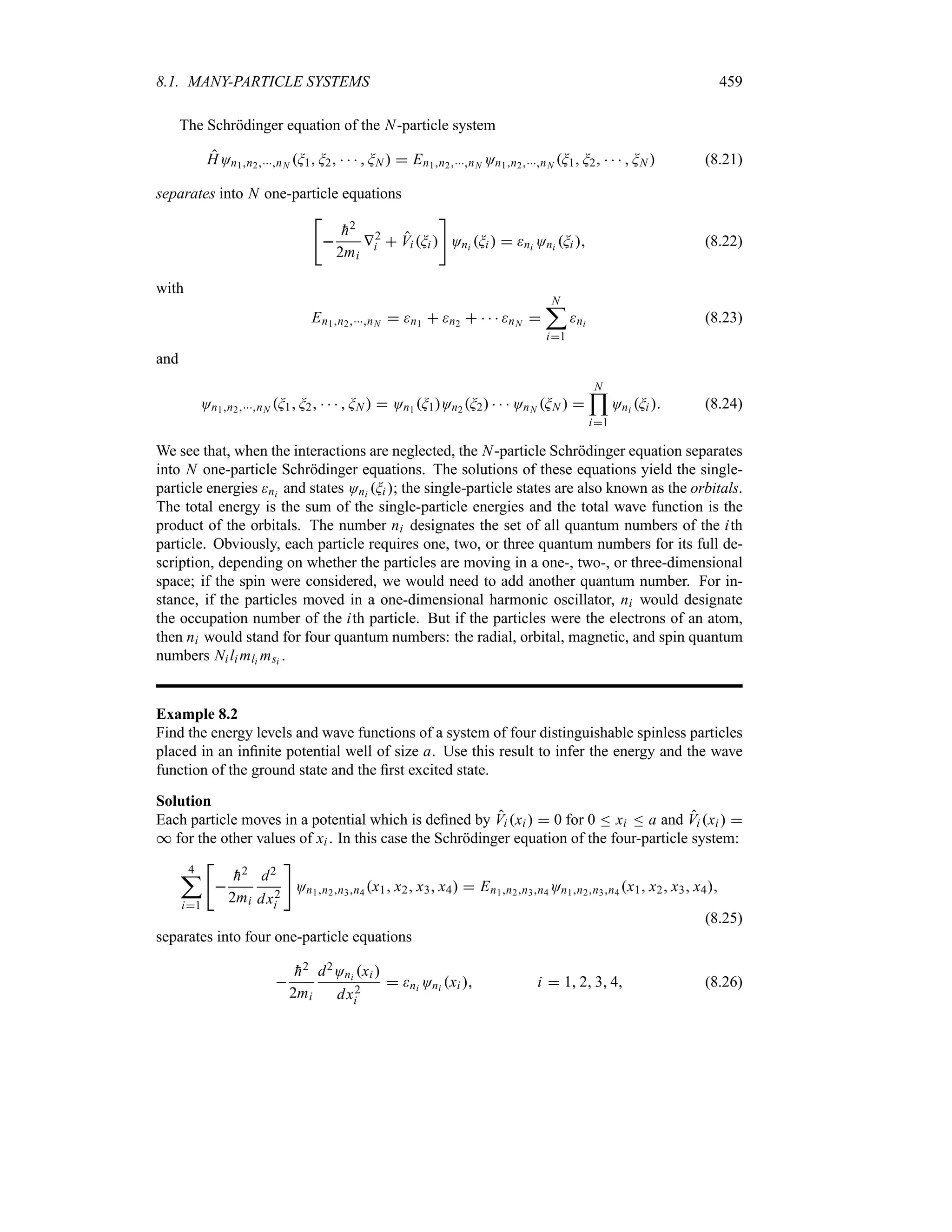
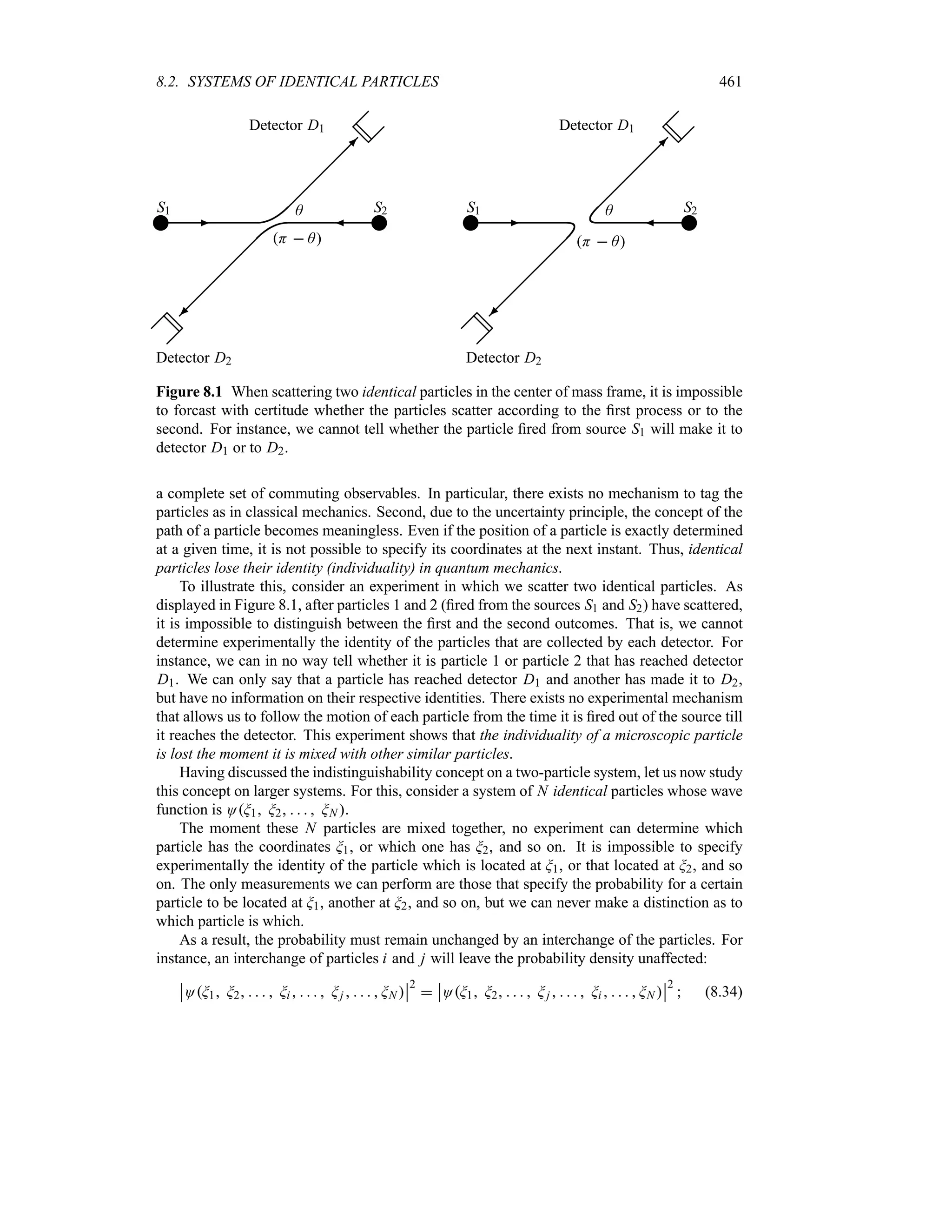
![8.2. SYSTEMS OF IDENTICAL PARTICLES 463
because V is invariant under the permutation of any pair of particles i z j:
VG1 Gi Gj GN VG1 Gj Gi GN (8.38)
This property can also be ascertained by showing that H commutes with the particle inter-
change operator Pi j . If O is eigenstate to H with eigenvalue E, we can write
H Pi j OG1 Gi Gj GN HOG1 Gj Gi GN
EOG1 Gj Gi GN E Pi j OG1 Gi Gj GN
Pi j EOG1 Gi Gj GN Pi j HOG1 Gi Gj GN
(8.39)
or
[H Pi j ] 0 (8.40)
Therefore, Pi j is a constant of the motion. That is, if we start with a wave function that is sym-
metric (antisymmetric), it will remain so for all subsequent times. Moreover, since Pi j and H
commute, they possess a complete set of functions that are joint eigenstates of both. As shown
in (8.15) to (8.17), these eigenstates have definite parity, either symmetric or antisymmetric.
8.2.3 Symmetrization Postulate
We have shown in (8.35) that the wave function of a system of N identical particles is either
symmetric or antisymmetric under the interchange of any pair of particles:
OG1 G2 Gi Gj GN OG1 G2 Gj Gi GN (8.41)
This result, which turns out to be supported by experimental evidence, is the very essence of
the symmetrization postulate which stipulates that, in nature, the states of systems containing
N identical particles are either totally symmetric or totally antisymmetric under the interchange
of any pair of particles and that states with mixed symmetry do not exist. Besides that, this
postulate states two more things:
Particles with integral spins, or bosons, have symmetric states.
Particles with half-odd-integral spins, or fermions, have antisymmetric states.
Fermions are said to obey Fermi–Dirac statistics and bosons to obey Bose–Einstein statistics.
So the wave function of a system of identical bosons is totally symmetric and the wave function
of a system of identical fermions is totally antisymmetric.
Composite particles
The foregoing discussion pertains to identical particles that are “simple” or elementary such as
quarks, electrons, positrons, muons, and so on. Let us now discuss the symmetry of systems
of identical composite “particles” where each particle is composed of two or more identical
elementary particles. For instance, alpha particles, which consist of nuclei that are composed
of two neutrons and two protons each, are a typical example of composite particles. A system
of N hydrogen atoms can also be viewed as a system of identical composite particles where
each “particle” (atom) consists of a proton and an electron. Protons, neutrons, pions, etc., are](https://image.slidesharecdn.com/zettili-250217213640-909f6141/75/Zettili-Quantum-mechanics-Concept-and-application-pdf-480-2048.jpg)


![472 CHAPTER 8. IDENTICAL PARTICLES
Table 8.1 Ground state electron configurations, spectroscopic description, and ionization en-
ergies for the first four rows of the periodic table. The brackets designate closed-shell elements.
Ground state Spectroscopic Ionization
Shell Z Element configuration description energy eV
1 1 H 1s1 2S12 13.60
2 He 1s2 1S0 24.58
2 3 Li [He]2s1 1s22s1 2S12 5.39
4 Be [He]2s2 1S0 9.32
5 B [He]2s22p1 2P12 8.30
6 C [He]2s22p2 3P0 11.26
7 N [He]2s22p3 4S32 14.55
8 O [He]2s22p4 3P2 13.61
9 F [He]2s22p5 2P32 17.42
10 Ne [He]2s22p6 1S0 21.56
3 11 Na [Ne]3s1 2S12 5.14
12 Mg [Ne]3s2 1S0 7.64
13 Al [Ne]3s23p1 2P12 5.94
14 Si [Ne]3s23p2 3P0 8.15
15 P [Ne]3s23p3 4S32 10.48
16 S [Ne]3s23p4 3P2 10.36
17 Cl [Ne]3s23p5 2P32 13.01
18 Ar [Ne]3s23p6 1S0 15.76
4 19 K [Ar]4s1 2S12 4.34
20 Ca [Ar]4s2 1S0 6.11
21 Sc [Ar]3d14s2 2D32 6.54
22 Ti [Ar]3d24s2 3F2 6.83
23 V [Ar]3d34s2 4F32 6.74
24 Cr [Ar]3d44s2 7S3 6.76
25 Mn [Ar]3d54s2 6S32 7.43
26 Fe [Ar]3d64s2 5D4 7.87
27 Co [Ar]3d74s2 4F92 7.86
28 Ni [Ar]3d84s2 3F4 7.63
29 Cu [Ar]3d104s1 2S12 7.72
30 Zn [Ar]3d104s2 1S0 9.39
31 Ga [Ar]3d104s24p1 2P12 6.00
32 Ge [Ar]3d104s24p2 3P0 7.88
33 As [Ar]3d104s24p3 4S32 9.81
34 Se [Ar]3d104s24p4 3P2 9.75
35 Br [Ar]3d104s24p5 2P32 11.84
36 Kr [Ar]3d104s24p6 1S0 9.81](https://image.slidesharecdn.com/zettili-250217213640-909f6141/75/Zettili-Quantum-mechanics-Concept-and-application-pdf-489-2048.jpg)
![474 CHAPTER 8. IDENTICAL PARTICLES
the nucleus, whereas the d-state electrons experience a much weaker attraction. This is known
as the screening effect, because the inner electrons, i.e., the s-state electrons, screen the nucleus;
hence the outward electrons (the d-state electrons) do not experience the full attraction of the
nucleus, but instead feel a weak effective potential. As a result, the energy of the 3d-state is
larger than that of the 4s-state. The screening effect also causes the energy of the 5s-state to
have a lower energy than the 4d-state, and so on. So for a given n, the energies Enl increase as
l increases; in fact, neglecting the spin–orbit interaction and considering relativistic corrections
we will show in Chapter 9 (9.90) that the ground state energy depends on the principal and
orbital quantum numbers n and l as E0
nl Z2 E0
n 1 :2 Z2[22l 1 34n]n , where
: 1137 is the fine structure constant and E0
n Rn2 136 eVn2.
In conclusion, the periodic table can be obtained by filling the orbitals in order of increasing
energy Enl as follows (Table 8.1):
1s2
2s2
2p6
3s2
3p6
4s2
3d10
4p6
5s2
4d10
5p6
6s2
4f14
5d10
6p6
7s2
5f14
6d10
7p6
(8.72)
Remarks
The chemical properties of an element is mostly determined by the outermost shell. Hence
elements with similar electron configurations for the outside shell have similar chemical prop-
erties. This is the idea behind the structure of the periodic table: it is arranged in a way that
all elements in a column have similar chemical properties. For example, the elements in the
last column, helium, neon, argon, krypton, and so on, have the outer p-shell completely filled
(except for helium whose outside shell is 1s). These atoms, which are formed when a shell or
a subshell is filled, are very stable, interact very weakly with one another, and do not combine
with other elements to form molecules or new compounds; that is, they are chemically inert.
They are very reluctant to give up or to accept an electron. Due to these properties, they are
called noble gases. They have a very low boiling point (around 200 iC). Note that each row
of the periodic table corresponds to filling out a shell or subshell of the atom, up to the next
noble gas. Also, there is a significant energy gap before the next level is encountered after each
of these elements. As shown in Table 8.1, a large energy is required to ionize these elements;
for instance, 2458 eV is needed to ionize a helium atom.
Atoms consisting of a closed shell (or a noble gas configuration) plus an s-electron (or a va-
lence electron), such as Li, Na, K, and so on, have the lowest binding energy; these elements are
known as the alkali metals. In elements consisting of an alkali configuration plus an electron,
the second s-electron is more bound than the valence electron of the alkali atom because of the
higher nuclear charge. As the p-shell is gradually filled (beyond the noble gas configuration),
the binding energy increases initially (as in boron, carbon, and nitrogen) till the fourth electron,
then it begins to drop (Table 8.1). This is due to the fact that when the p-shell is less than half
full all spins are parallel; hence all three spatial wave functions are antisymmetric. With the
fourth electron (as in oxygen), two spins will be antiparallel or paired; hence the spatial wave
function is not totally antisymmetric, causing a drop in the energy. Note that elements with
one electron more than or one electron less than noble gas configurations are the most active
chemically, because they tend to easily give up or easily accept one electron.
Example 8.4
(a) Specify the total angular momenta corresponding to 4G, 3H, and 1D.](https://image.slidesharecdn.com/zettili-250217213640-909f6141/75/Zettili-Quantum-mechanics-Concept-and-application-pdf-491-2048.jpg)
![8.5. SOLVED PROBLEMS 475
(b) Find the spectroscopic notation for the ground state configurations of aluminum Al
(Z 13) and scandium Sc (Z 21).
Solution
(a) For the term 4G the orbital angular momentum is L 4 and the spin is S 32, since
2S 1 4. The values of the total angular momentum corresponding to the coupling of L 4
and S 32 are given by 4 32 n J n 4 32. Hence we have J 52, 72, 92, 112.
Similarly, for 3H we have S 1 and L 5. Therefore, we have 5 1 n J n 5 1, or
J 4, 5, 6.
For 1D we have S 0 and L 2. Therefore, we have 2 0 n J n 2 0, or J 2.
(b) The ground state configuration of Al is [Ne]3s23p1. The total angular momentum
of this element is determined by the 3p electron, because S 0 and L 0 for both [Ne] and
3s2. Since the 3p electron has S 12 and L 1, the total angular momentum is given by
1 12 n J n 1 12. Hence we have J 12, 32. Which of the values J 12 and
J 32 has a lower energy? According to Hund’s third rule, since the 3p shell is less than half
full, the state J L S 12 has the lower energy. Hence the ground state configuration
of Al corresponds to 2P12 (Table 8.1), where we have used the spectroscopic notation 2S1LJ .
Since the ground state configuration of Sc is [Ar]4s23d1, the angular momentum is given
by that of the 3d electron. Since S 12 and L 2, and since the 3d shell is less than half
full, Hund’s third rule dictates that the total angular momentum is given by J L S
2 12 32. Hence we have 2D32.
8.5 Solved Problems
Problem 8.1
Consider a system of three noninteracting particles that are confined to move in a one-dimensional
infinite potential well of length a: Vx 0 for 0 x a and Vx * for other values of
x. Determine the energy and wave function of the ground state and the first and second excited
states when the three particles are (a) spinless and distinguishable with m1 m2 m3; (b)
identical bosons; (c) identical spin 1
2 particles; and (d) distinguishable spin 1
2 particles.
Solution
(a) As shown in Example 8.2 on page 459, the total energy and wave function are given by
En1n2n3
h2H2
2a2
‚
n2
1
m1
n2
2
m2
n2
3
m3
(8.73)
On1n2n3 x1 x2 x3
U
8
a3
sin
rn1H
a
x1
s
sin
rn2H
a
x2
s
sin
rn3H
a
x3
s
(8.74)
The ground state of the system corresponds to the case where all three particles occupy their
respective ground state orbitals, n1 n2 n3 1; hence
E0
E111
h2H2
2a2
t
1
m1
1
m2
1
m3
u
(8.75)
O0
x1 x2 x3 O111x1 x2 x3
U
8
a3
sin
rH
a
x1
s
sin
rH
a
x2
s
sin
rH
a
x3
s
(8.76)](https://image.slidesharecdn.com/zettili-250217213640-909f6141/75/Zettili-Quantum-mechanics-Concept-and-application-pdf-492-2048.jpg)