Reservoir Engineering 1 Course (2nd Ed.)
1. Multiple-Phase Flow
2. Pressure Disturbance in Reservoirs
3. USS Flow Regime
A. USS: Mathematical Formulation

4. Diffusivity Equation
A. Solution of Diffusivity Equation
a.

Ei- Function Solution
1. Solutions of Diffusivity Equation
A. pD Solution
B. Analytical Solution

2. USS(LT) Regime for Radial flow of SC Fluids:
Finite-Radial Reservoir
3. Relation between pD and Ei
4. USS Regime for Radial Flow of C Fluids
A. (Exact Method)
B. (P2 Approximation Method)
C. (P Approximation Method)

5. PSS regime Flow Constant
The Dimensionless Pressure Drop (pD)
Solution
The second form of solution to the diffusivity
equation is called the dimensionless pressure drop.
Well test analysis often makes use of the concept
of the dimensionless variables in solving the
unsteady-state flow equation.
The importance of dimensionless variables is that they
simplify the diffusivity equation and its solution by
combining the reservoir parameters (such as
permeability, porosity, etc.) and thereby reduce the total
number of unknowns.

Fall 13 H. AlamiNia

Reservoir Engineering 1 Course (2nd Ed.)

5
Dimensionless Pressure Drop Solution
Introduction
To introduce the concept of the dimensionless
pressure drop solution, consider for example
Darcy’s equation in a radial form as given previously
by:

Rearrange the above equation to give:

Fall 13 H. AlamiNia

Reservoir Engineering 1 Course (2nd Ed.)

6
Dimensionless Pressure
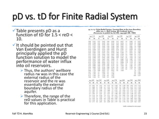
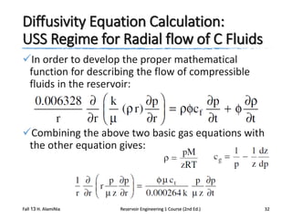
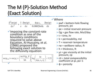
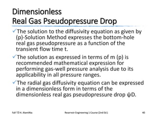
It is obvious that the right hand side of the above
equation has no units (i.e., dimensionless) and,
accordingly, the left-hand side must be
dimensionless.
Since the left-hand side is dimensionless, and (pe −
pwf) has the units of psi, it follows that the term
[Qo Bo μo/ (0.00708kh)] has units of pressure.


Fall 13 H. AlamiNia

Reservoir Engineering 1 Course (2nd Ed.)

7
pD in Transient Flow Analysis
In transient flow analysis, the dimensionless
pressure pD is always a function of dimensionless
time that is defined by the following expression:

Fall 13 H. AlamiNia

Reservoir Engineering 1 Course (2nd Ed.)

8
Dimensionless Time
In transient flow analysis, the dimensionless pressure pD is
always a function of dimensionless time that is defined by
the following expression:

The above expression is only one form of the dimensionless
time.
Another definition in common usage is tDA, the
dimensionless time based on total drainage area.

Where A = total drainage area = π re^2, re = drainage radius,
ft, rw = wellbore radius, ft
Fall 13 H. AlamiNia

Reservoir Engineering 1 Course (2nd Ed.)

9
Dimensionless Radial Distances
The dimensionless
pressure pD also varies
with location in the
reservoir as
represented by the
dimensionless radial
distances rD and reD
that are defined by:

Fall 13 H. AlamiNia

Where
pD = dimensionless
pressure drop
reD = dimensionless
external radius
tD = dimensionless time
rD = dimensionless
radius
t = time, hr
p(r, t) = pressure at
radius r and time t
k = permeability, md
μ = viscosity, cp

Reservoir Engineering 1 Course (2nd Ed.)

10
Dimensionless Diffusivity Equation
The above dimensionless groups
(i.e., pD, tD, and rD)
can be introduced into the diffusivity equation to
transform the equation into the following
dimensionless form:

Fall 13 H. AlamiNia

Reservoir Engineering 1 Course (2nd Ed.)

11
Analytical Solution Assumptions
Van Everdingen and Hurst (1949) proposed an
analytical solution to the dimensionless diffusivity
equation by assuming:
Perfectly radial reservoir system
The producing well is in the center and producing at a
constant production rate of Q
Uniform pressure pi throughout the reservoir before
production
No flow across the external radius re

Fall 13 H. AlamiNia

Reservoir Engineering 1 Course (2nd Ed.)

13
Van Everdingen and Hurst Solution
Van Everdingen and Hurst presented the solution to
the in a form of infinite series of exponential terms
and Bessel functions.
The authors evaluated this series for several values of
reD over a wide range of values for tD.

Chatas (1953) and Lee (1982) conveniently
tabulated these solutions for the following two
cases:
Infinite-acting reservoir
Finite-radial reservoir

Fall 13 H. AlamiNia

Reservoir Engineering 1 Course (2nd Ed.)

14
Infinite-Acting Reservoir
When a well is put on production at a constant flow
rate after a shut-in period, the pressure in the
wellbore begins to drop and causes a pressure
disturbance to spread in the reservoir.
The influence of the reservoir boundaries or the shape
of the drainage area does not affect the rate at which
the pressure disturbance spreads in the formation.

That is why the transient state flow is also called
the infinite acting state.

Fall 13 H. AlamiNia

Reservoir Engineering 1 Course (2nd Ed.)

15
Parameters Affecting Pwf
during Infinite Acting Period
During the infinite acting period, the declining rate
of wellbore pressure and the manner by which the
pressure disturbance spreads through the reservoir
are determined by reservoir and fluid
characteristics such as:
Porosity, φ
Permeability, k
Total compressibility, ct
Viscosity, μ

Fall 13 H. AlamiNia

Reservoir Engineering 1 Course (2nd Ed.)

16
pD Values for
the Infinite-Acting Reservoir
For an infinite-acting
reservoir, i.e., reD = ∞,
the dimensionless
pressure drop function
pD is strictly a function
of the dimensionless
time tD, or:
Chatas and Lee
tabulated the pD values
for the infinite-acting
reservoir.
Fall 13 H. AlamiNia

Reservoir Engineering 1 Course (2nd Ed.)

17
pD Approximation
for the Infinite-Acting Reservoir
The following mathematical expressions can be
used to approximate these tabulated values of pD:
For tD < 0.01:

For tD > 100:

For 0.02 < tD < 1000:

Fall 13 H. AlamiNia

Reservoir Engineering 1 Course (2nd Ed.)

18
Finite-Radial Reservoir
The arrival of the pressure disturbance at the well
drainage boundary marks the end of the transient
flow period and the beginning of the semi
(pseudo)-steady state.
During this flow state, the reservoir boundaries and the
shape of the drainage area influence the wellbore
pressure response as well as the behavior of the
pressure distribution throughout the reservoir.

Fall 13 H. AlamiNia

Reservoir Engineering 1 Course (2nd Ed.)

20
Late-Transient State
Intuitively, one should not expect the change from
the transient to the semi-steady state in this
bounded (finite) system to occur instantaneously.
There is a short period of time that separates the
transient state from the semi-steady state that is called
late-transient state.

Due to its complexity and short duration, the late
transient flow is not used in practical well test
analysis.

Fall 13 H. AlamiNia

Reservoir Engineering 1 Course (2nd Ed.)

21
pD for a Finite Radial System
For a finite radial system, the pD-function is a
function of both the dimensionless time and radius,
or:

Fall 13 H. AlamiNia

Reservoir Engineering 1 Course (2nd Ed.)

22
pD vs. tD for Finite Radial System
Table presents pD as a
function of tD for 1.5 < reD <
10.
It should be pointed out that
Van Everdingen and Hurst
principally applied the pD
function solution to model the
performance of water influx
into oil reservoirs.
 Thus, the authors’ wellbore
radius rw was in this case the
external radius of the
reservoir and the re was
essentially the external
boundary radius of the
aquifer.
 Therefore, the range of the
reD values in Table is practical
for this application.

Fall 13 H. AlamiNia

Reservoir Engineering 1 Course (2nd Ed.)

23
pD Calculation
Chatas (1953) proposed the following
mathematical expression for calculating pD:

A special case of above Equation arises when
(reD) ^2>> 1, then:

Fall 13 H. AlamiNia

Reservoir Engineering 1 Course (2nd Ed.)

24
Using the pD-Function
in Pwf Determination
The computational procedure of using the pD-function
in determining the bottom-hole flowing pressure
changing the transient flow period is summarized in the
following steps:
Step 1. Calculate the dimensionless time tD
Step 2. Calculate the dimensionless radius reD
Step 3. Using the calculated values of tD and reD,
determine the corresponding pressure function pD
from the appropriate table or equation.
Step 4. Solve for the pressure at the desired radius, i.e.,
rw
Fall 13 H. AlamiNia

Reservoir Engineering 1 Course (2nd Ed.)

25
pD-Function vs. Ei-Function Technique
The solution as given by the pD-function technique
is identical to that of the Ei-function approach.
The main difference between the two formulations
is that the pD-function can be used only to calculate
the pressure at radius r when the flow rate Q is
constant and known.
In that case, the pD-function application is essentially restricted
to the wellbore radius because the rate is usually known.

On the other hand, the Ei-function approach can be
used to calculate the pressure at any radius in the
reservoir by using the well flow rate Q.
Fall 13 H. AlamiNia

Reservoir Engineering 1 Course (2nd Ed.)

27
pD Application
In transient flow testing, we normally record the
bottom-hole flowing pressure as a function of time.
Therefore, the dimensionless pressure drop technique
can be used to determine one or more of the reservoir
properties, e.g., k or kh.

Fall 13 H. AlamiNia

Reservoir Engineering 1 Course (2nd Ed.)

28
Relation between pD & Ei for Td>100
It should be pointed out that,
for an infinite-acting reservoir with tD > 100,
the pD-function is related to the Ei-function by the following
relation:

Fall 13 H. AlamiNia

Reservoir Engineering 1 Course (2nd Ed.)

29
Diffusivity Equation
Gas viscosity and density vary significantly with
pressure and
therefore the assumptions of diffusivity equation are not
satisfied for gas systems, i.e., compressible fluids.

Fall 13 H. AlamiNia

Reservoir Engineering 1 Course (2nd Ed.)

31
Diffusivity Equation Calculation:
USS Regime for Radial flow of C Fluids
In order to develop the proper mathematical
function for describing the flow of compressible
fluids in the reservoir:

Combining the above two basic gas equations with
the other equation gives:

Fall 13 H. AlamiNia

Reservoir Engineering 1 Course (2nd Ed.)

32
Using M (P) for Radial Equation for
Compressible Fluids
Al-Hussainy, Ramey, and Crawford (1966) linearize
the above basic flow equation by introducing the
real gas potential m (p).

Combining above equation with below yields the
radial equation for compressible fluids:

Fall 13 H. AlamiNia

Reservoir Engineering 1 Course (2nd Ed.)

33
Exact Solution of the Equation for
Compressible Fluids
The radial diffusivity equation for compressible
fluids relates the real gas pseudopressure (real gas
potential) to the time t and the radius r.
Al-Hussainy, Ramey, and Crawford (1966) pointed
out that in gas well testing analysis, the constantrate solution has more practical applications than
that provided by the constant pressure solution.
The authors provided the exact solution to the Equation
that is commonly referred to as the m (p)-solution
method.

Fall 13 H. AlamiNia

Reservoir Engineering 1 Course (2nd Ed.)

34
Solution Forms of the Equation for
Compressible Fluids
There are also two other solutions that
approximate the exact solution.
In general, there are three forms of the
mathematical solution to the diffusivity equation:
The m (p)-Solution Method (Exact Solution)
The Pressure-Squared Method (p2-Approximation
Method)
The Pressure Method (p-Approximation Method)

Fall 13 H. AlamiNia

Reservoir Engineering 1 Course (2nd Ed.)

35
The M (P)-Solution Method
(Exact Solution)
Where

Imposing the constant-rate
condition as one of the
boundary conditions
required to solve above
Equation, Al-Hussainy, et al.
(1966) proposed the
following exact solution to
the diffusivity equation:


Fall 13 H. AlamiNia

 pwf = bottom-hole flowing
pressure, psi
 pe = initial reservoir pressure
 Qg = gas flow rate, Mscf/day
 t = time, hr
 k = permeability, md
 T = reservoir temperature
 rw = wellbore radius, ft
 h = thickness, ft
 μi = gas viscosity at the initial
pressure, cp
 cti = total compressibility
coefficient at pi, psi−1
 φ = porosity

Reservoir Engineering 1 Course (2nd Ed.)

36
The M (P)-Solution Method
in Terms of the tD
The m (p)-Solution Equation can be written
equivalently in terms of the dimensionless time tD
as:

The dimensionless time is defined previously as:

The parameter γ is called Euler’s constant and given
by:
Fall 13 H. AlamiNia

Reservoir Engineering 1 Course (2nd Ed.)

37
Dimensionless
Real Gas Pseudopressure Drop
The solution to the diffusivity equation as given by
(p)-Solution Method expresses the bottom-hole
real gas pseudopressure as a function of the
transient flow time t.
The solution as expressed in terms of m (p) is
recommended mathematical expression for
performing gas-well pressure analysis due to its
applicability in all pressure ranges.
The radial gas diffusivity equation can be expressed
in a dimensionless form in terms of the
dimensionless real gas pseudopressure drop ψD.
Fall 13 H. AlamiNia

Reservoir Engineering 1 Course (2nd Ed.)

40
Solution of Dimensionless Equation
The solution to the dimensionless equation is given
by:

The dimensionless pseudopressure drop ψD can be
determined as a function of tD by using the appropriate
expressions.
When tD > 100, the ψD can be calculated by:

Fall 13 H. AlamiNia

Reservoir Engineering 1 Course (2nd Ed.)

41
The Pressure-Squared Method
(P2-Approximation Method)
The first approximation to the exact solution is to
remove the pressure- dependent term (μz) outside
the integral that defines m (pwf) and m (pi) to give:

The bars over μ and z represent the values of the
gas viscosity and deviation factor as evaluated at
the average pressure p–. This average pressure is
given by:

Fall 13 H. AlamiNia

Reservoir Engineering 1 Course (2nd Ed.)

42
Converting M (P)-Solution Method
to P2-Approximation
Combining Equations:

Fall 13 H. AlamiNia

Reservoir Engineering 1 Course (2nd Ed.)

43
P2-Approximation Assumptions
The Pressure-Squared Method solution forms
indicate that the product (μz) is assumed constant
at the average pressure p–.
 This effectively limits the applicability of the p2-method
to reservoir pressures < 2000.
It should be pointed out that when the p2-method is
used to determine pwf it is perhaps sufficient to set μ–
z– = μi z.

Fall 13 H. AlamiNia

Reservoir Engineering 1 Course (2nd Ed.)

44
The Pressure Method
(P-Approximation Method)
The second method of approximation to the exact
solution of the radial flow of gases is to treat the
gas as a pseudoliquid.

Fall 13 H. AlamiNia

Reservoir Engineering 1 Course (2nd Ed.)

46
The Pressure Method Equation
Fetkovich (1973)
suggested that at high
pressures (p > 3000),
1/μBg is nearly
constant as shown
schematically in Figure.
Imposing Fetkovich’s
condition gives:

Fall 13 H. AlamiNia

Reservoir Engineering 1 Course (2nd Ed.)

47
Converting M (P)-Solution Method
to P-Approximation
Combining Equations:

Fall 13 H. AlamiNia

Reservoir Engineering 1 Course (2nd Ed.)

48
Average Pressure
in P-Approximation Method
It should be noted that the gas properties, i.e., μ,
Bg, and ct, are evaluated at pressure p– as defined
below:
Again, this method is only limited to applications
above 3000 psi.
When solving for pwf, it might be sufficient to evaluate
the gas properties at pi.

Fall 13 H. AlamiNia

Reservoir Engineering 1 Course (2nd Ed.)

49
Flash Back: USS
In the unsteady-state flow cases discussed
previously, it was assumed that a well is located in a
very large reservoir and producing at a constant
flow rate.
This rate creates a pressure disturbance in the reservoir
that travels throughout this infinite-size reservoir.
During this transient flow period, reservoir boundaries
have no effect on the pressure behavior of the well.
Obviously, the time period where this assumption can be
imposed is often very short in length.

Fall 13 H. AlamiNia

Reservoir Engineering 1 Course (2nd Ed.)

51
Pseudosteady (Semisteady)-State
Flow Regime
As soon as the pressure disturbance reaches all
drainage boundaries, it ends the transient
(unsteady-state) flow regime.
A different flow regime begins that is called
pseudosteady (semisteady)-state flow.
It is necessary at this point to impose different
boundary conditions on the diffusivity equation and
derive an appropriate solution to this flow regime.

Fall 13 H. AlamiNia

Reservoir Engineering 1 Course (2nd Ed.)

52
Semisteady-State Flow Regime
Figure shows a well in radial
system that is producing at
a constant rate for a long
enough period that
eventually affects the entire
drainage area.
During this semisteadystate flow, the change in
pressure with time
becomes the same
throughout the drainage
area.
Section B shows that the
pressure distributions
become paralleled at
successive time periods.
Fall 13 H. AlamiNia

Reservoir Engineering 1 Course (2nd Ed.)

53
PSS Constant
The important PSS condition can be expressed as:

The constant referred to in the above equation can
be obtained from a simple material balance using
the definition of the compressibility, thus:

Fall 13 H. AlamiNia

Reservoir Engineering 1 Course (2nd Ed.)

54
Pressure Decline Rate
Expressing the pressure decline rate dp/dt in the
above relation in psi/hr gives:

Where q = flow rate, bbl/day
Qo = flow rate, STB/day
dp/dt = pressure decline rate, psi/hr
V = pore volume, bbl

Fall 13 H. AlamiNia

Reservoir Engineering 1 Course (2nd Ed.)

55
Pressure Decline Rate
for Radial Drainage System
For a radial drainage system, the pore volume is
given by:

Where A = drainage area, ft2

Fall 13 H. AlamiNia

Reservoir Engineering 1 Course (2nd Ed.)

56
Characteristics of
the Pressure Behavior during PSS
Examination reveals the following important
characteristics of the behavior of the pressure
decline rate dp/dt during the semisteady-state flow:
The reservoir pressure declines at a higher rate with an
increase in the fluids production rate
The reservoir pressure declines at a slower rate for
reservoirs with higher total compressibility coefficients
The reservoir pressure declines at a lower rate for
reservoirs with larger pore volumes

Fall 13 H. AlamiNia

Reservoir Engineering 1 Course (2nd Ed.)

57
Semisteady-State Condition
Matthews, Brons, and Hazebroek (1954) pointed
out that once the reservoir is producing under the
semisteady-state condition,
Each well will drain from within its own no-flow
boundary independently of the other wells.

For this condition to prevail:
 The pressure decline rate dp/dt must be approximately
constant throughout the entire reservoir,
Otherwise, flow would occur across the boundaries
causing a readjustment in their positions.

Fall 13 H. AlamiNia

Reservoir Engineering 1 Course (2nd Ed.)

58
1. Ahmed, T. (2010). Reservoir engineering
handbook (Gulf Professional Publishing).
Chapter 6
1. PSS Regime
A.
B.
C.
D.

Average Reservoir Pressure
PSS regime for Radial Flow of SC Fluids
Effect of Well Location within the Drainage Area
PSS Regime for Radial Flow of C Fluids

2. Skin Concept
3. Using S for Radial Flow in Flow Equations
4. Turbulent Flow
Q921 re1 lec8 v1

Q921 re1 lec8 v1

  • 1.
    Reservoir Engineering 1Course (2nd Ed.)
  • 2.
    1. Multiple-Phase Flow 2.Pressure Disturbance in Reservoirs 3. USS Flow Regime A. USS: Mathematical Formulation 4. Diffusivity Equation A. Solution of Diffusivity Equation a. Ei- Function Solution
  • 3.
    1. Solutions ofDiffusivity Equation A. pD Solution B. Analytical Solution 2. USS(LT) Regime for Radial flow of SC Fluids: Finite-Radial Reservoir 3. Relation between pD and Ei 4. USS Regime for Radial Flow of C Fluids A. (Exact Method) B. (P2 Approximation Method) C. (P Approximation Method) 5. PSS regime Flow Constant
  • 5.
    The Dimensionless PressureDrop (pD) Solution The second form of solution to the diffusivity equation is called the dimensionless pressure drop. Well test analysis often makes use of the concept of the dimensionless variables in solving the unsteady-state flow equation. The importance of dimensionless variables is that they simplify the diffusivity equation and its solution by combining the reservoir parameters (such as permeability, porosity, etc.) and thereby reduce the total number of unknowns. Fall 13 H. AlamiNia Reservoir Engineering 1 Course (2nd Ed.) 5
  • 6.
    Dimensionless Pressure DropSolution Introduction To introduce the concept of the dimensionless pressure drop solution, consider for example Darcy’s equation in a radial form as given previously by: Rearrange the above equation to give: Fall 13 H. AlamiNia Reservoir Engineering 1 Course (2nd Ed.) 6
  • 7.
    Dimensionless Pressure It isobvious that the right hand side of the above equation has no units (i.e., dimensionless) and, accordingly, the left-hand side must be dimensionless. Since the left-hand side is dimensionless, and (pe − pwf) has the units of psi, it follows that the term [Qo Bo μo/ (0.00708kh)] has units of pressure.  Fall 13 H. AlamiNia Reservoir Engineering 1 Course (2nd Ed.) 7
  • 8.
    pD in TransientFlow Analysis In transient flow analysis, the dimensionless pressure pD is always a function of dimensionless time that is defined by the following expression: Fall 13 H. AlamiNia Reservoir Engineering 1 Course (2nd Ed.) 8
  • 9.
    Dimensionless Time In transientflow analysis, the dimensionless pressure pD is always a function of dimensionless time that is defined by the following expression: The above expression is only one form of the dimensionless time. Another definition in common usage is tDA, the dimensionless time based on total drainage area. Where A = total drainage area = π re^2, re = drainage radius, ft, rw = wellbore radius, ft Fall 13 H. AlamiNia Reservoir Engineering 1 Course (2nd Ed.) 9
  • 10.
    Dimensionless Radial Distances Thedimensionless pressure pD also varies with location in the reservoir as represented by the dimensionless radial distances rD and reD that are defined by: Fall 13 H. AlamiNia Where pD = dimensionless pressure drop reD = dimensionless external radius tD = dimensionless time rD = dimensionless radius t = time, hr p(r, t) = pressure at radius r and time t k = permeability, md μ = viscosity, cp Reservoir Engineering 1 Course (2nd Ed.) 10
  • 11.
    Dimensionless Diffusivity Equation Theabove dimensionless groups (i.e., pD, tD, and rD) can be introduced into the diffusivity equation to transform the equation into the following dimensionless form: Fall 13 H. AlamiNia Reservoir Engineering 1 Course (2nd Ed.) 11
  • 13.
    Analytical Solution Assumptions VanEverdingen and Hurst (1949) proposed an analytical solution to the dimensionless diffusivity equation by assuming: Perfectly radial reservoir system The producing well is in the center and producing at a constant production rate of Q Uniform pressure pi throughout the reservoir before production No flow across the external radius re Fall 13 H. AlamiNia Reservoir Engineering 1 Course (2nd Ed.) 13
  • 14.
    Van Everdingen andHurst Solution Van Everdingen and Hurst presented the solution to the in a form of infinite series of exponential terms and Bessel functions. The authors evaluated this series for several values of reD over a wide range of values for tD. Chatas (1953) and Lee (1982) conveniently tabulated these solutions for the following two cases: Infinite-acting reservoir Finite-radial reservoir Fall 13 H. AlamiNia Reservoir Engineering 1 Course (2nd Ed.) 14
  • 15.
    Infinite-Acting Reservoir When awell is put on production at a constant flow rate after a shut-in period, the pressure in the wellbore begins to drop and causes a pressure disturbance to spread in the reservoir. The influence of the reservoir boundaries or the shape of the drainage area does not affect the rate at which the pressure disturbance spreads in the formation. That is why the transient state flow is also called the infinite acting state. Fall 13 H. AlamiNia Reservoir Engineering 1 Course (2nd Ed.) 15
  • 16.
    Parameters Affecting Pwf duringInfinite Acting Period During the infinite acting period, the declining rate of wellbore pressure and the manner by which the pressure disturbance spreads through the reservoir are determined by reservoir and fluid characteristics such as: Porosity, φ Permeability, k Total compressibility, ct Viscosity, μ Fall 13 H. AlamiNia Reservoir Engineering 1 Course (2nd Ed.) 16
  • 17.
    pD Values for theInfinite-Acting Reservoir For an infinite-acting reservoir, i.e., reD = ∞, the dimensionless pressure drop function pD is strictly a function of the dimensionless time tD, or: Chatas and Lee tabulated the pD values for the infinite-acting reservoir. Fall 13 H. AlamiNia Reservoir Engineering 1 Course (2nd Ed.) 17
  • 18.
    pD Approximation for theInfinite-Acting Reservoir The following mathematical expressions can be used to approximate these tabulated values of pD: For tD < 0.01: For tD > 100: For 0.02 < tD < 1000: Fall 13 H. AlamiNia Reservoir Engineering 1 Course (2nd Ed.) 18
  • 20.
    Finite-Radial Reservoir The arrivalof the pressure disturbance at the well drainage boundary marks the end of the transient flow period and the beginning of the semi (pseudo)-steady state. During this flow state, the reservoir boundaries and the shape of the drainage area influence the wellbore pressure response as well as the behavior of the pressure distribution throughout the reservoir. Fall 13 H. AlamiNia Reservoir Engineering 1 Course (2nd Ed.) 20
  • 21.
    Late-Transient State Intuitively, oneshould not expect the change from the transient to the semi-steady state in this bounded (finite) system to occur instantaneously. There is a short period of time that separates the transient state from the semi-steady state that is called late-transient state. Due to its complexity and short duration, the late transient flow is not used in practical well test analysis. Fall 13 H. AlamiNia Reservoir Engineering 1 Course (2nd Ed.) 21
  • 22.
    pD for aFinite Radial System For a finite radial system, the pD-function is a function of both the dimensionless time and radius, or: Fall 13 H. AlamiNia Reservoir Engineering 1 Course (2nd Ed.) 22
  • 23.
    pD vs. tDfor Finite Radial System Table presents pD as a function of tD for 1.5 < reD < 10. It should be pointed out that Van Everdingen and Hurst principally applied the pD function solution to model the performance of water influx into oil reservoirs.  Thus, the authors’ wellbore radius rw was in this case the external radius of the reservoir and the re was essentially the external boundary radius of the aquifer.  Therefore, the range of the reD values in Table is practical for this application. Fall 13 H. AlamiNia Reservoir Engineering 1 Course (2nd Ed.) 23
  • 24.
    pD Calculation Chatas (1953)proposed the following mathematical expression for calculating pD: A special case of above Equation arises when (reD) ^2>> 1, then: Fall 13 H. AlamiNia Reservoir Engineering 1 Course (2nd Ed.) 24
  • 25.
    Using the pD-Function inPwf Determination The computational procedure of using the pD-function in determining the bottom-hole flowing pressure changing the transient flow period is summarized in the following steps: Step 1. Calculate the dimensionless time tD Step 2. Calculate the dimensionless radius reD Step 3. Using the calculated values of tD and reD, determine the corresponding pressure function pD from the appropriate table or equation. Step 4. Solve for the pressure at the desired radius, i.e., rw Fall 13 H. AlamiNia Reservoir Engineering 1 Course (2nd Ed.) 25
  • 27.
    pD-Function vs. Ei-FunctionTechnique The solution as given by the pD-function technique is identical to that of the Ei-function approach. The main difference between the two formulations is that the pD-function can be used only to calculate the pressure at radius r when the flow rate Q is constant and known. In that case, the pD-function application is essentially restricted to the wellbore radius because the rate is usually known. On the other hand, the Ei-function approach can be used to calculate the pressure at any radius in the reservoir by using the well flow rate Q. Fall 13 H. AlamiNia Reservoir Engineering 1 Course (2nd Ed.) 27
  • 28.
    pD Application In transientflow testing, we normally record the bottom-hole flowing pressure as a function of time. Therefore, the dimensionless pressure drop technique can be used to determine one or more of the reservoir properties, e.g., k or kh. Fall 13 H. AlamiNia Reservoir Engineering 1 Course (2nd Ed.) 28
  • 29.
    Relation between pD& Ei for Td>100 It should be pointed out that, for an infinite-acting reservoir with tD > 100, the pD-function is related to the Ei-function by the following relation: Fall 13 H. AlamiNia Reservoir Engineering 1 Course (2nd Ed.) 29
  • 31.
    Diffusivity Equation Gas viscosityand density vary significantly with pressure and therefore the assumptions of diffusivity equation are not satisfied for gas systems, i.e., compressible fluids. Fall 13 H. AlamiNia Reservoir Engineering 1 Course (2nd Ed.) 31
  • 32.
    Diffusivity Equation Calculation: USSRegime for Radial flow of C Fluids In order to develop the proper mathematical function for describing the flow of compressible fluids in the reservoir: Combining the above two basic gas equations with the other equation gives: Fall 13 H. AlamiNia Reservoir Engineering 1 Course (2nd Ed.) 32
  • 33.
    Using M (P)for Radial Equation for Compressible Fluids Al-Hussainy, Ramey, and Crawford (1966) linearize the above basic flow equation by introducing the real gas potential m (p). Combining above equation with below yields the radial equation for compressible fluids: Fall 13 H. AlamiNia Reservoir Engineering 1 Course (2nd Ed.) 33
  • 34.
    Exact Solution ofthe Equation for Compressible Fluids The radial diffusivity equation for compressible fluids relates the real gas pseudopressure (real gas potential) to the time t and the radius r. Al-Hussainy, Ramey, and Crawford (1966) pointed out that in gas well testing analysis, the constantrate solution has more practical applications than that provided by the constant pressure solution. The authors provided the exact solution to the Equation that is commonly referred to as the m (p)-solution method. Fall 13 H. AlamiNia Reservoir Engineering 1 Course (2nd Ed.) 34
  • 35.
    Solution Forms ofthe Equation for Compressible Fluids There are also two other solutions that approximate the exact solution. In general, there are three forms of the mathematical solution to the diffusivity equation: The m (p)-Solution Method (Exact Solution) The Pressure-Squared Method (p2-Approximation Method) The Pressure Method (p-Approximation Method) Fall 13 H. AlamiNia Reservoir Engineering 1 Course (2nd Ed.) 35
  • 36.
    The M (P)-SolutionMethod (Exact Solution) Where Imposing the constant-rate condition as one of the boundary conditions required to solve above Equation, Al-Hussainy, et al. (1966) proposed the following exact solution to the diffusivity equation:  Fall 13 H. AlamiNia  pwf = bottom-hole flowing pressure, psi  pe = initial reservoir pressure  Qg = gas flow rate, Mscf/day  t = time, hr  k = permeability, md  T = reservoir temperature  rw = wellbore radius, ft  h = thickness, ft  μi = gas viscosity at the initial pressure, cp  cti = total compressibility coefficient at pi, psi−1  φ = porosity Reservoir Engineering 1 Course (2nd Ed.) 36
  • 37.
    The M (P)-SolutionMethod in Terms of the tD The m (p)-Solution Equation can be written equivalently in terms of the dimensionless time tD as: The dimensionless time is defined previously as: The parameter γ is called Euler’s constant and given by: Fall 13 H. AlamiNia Reservoir Engineering 1 Course (2nd Ed.) 37
  • 40.
    Dimensionless Real Gas PseudopressureDrop The solution to the diffusivity equation as given by (p)-Solution Method expresses the bottom-hole real gas pseudopressure as a function of the transient flow time t. The solution as expressed in terms of m (p) is recommended mathematical expression for performing gas-well pressure analysis due to its applicability in all pressure ranges. The radial gas diffusivity equation can be expressed in a dimensionless form in terms of the dimensionless real gas pseudopressure drop ψD. Fall 13 H. AlamiNia Reservoir Engineering 1 Course (2nd Ed.) 40
  • 41.
    Solution of DimensionlessEquation The solution to the dimensionless equation is given by: The dimensionless pseudopressure drop ψD can be determined as a function of tD by using the appropriate expressions. When tD > 100, the ψD can be calculated by: Fall 13 H. AlamiNia Reservoir Engineering 1 Course (2nd Ed.) 41
  • 42.
    The Pressure-Squared Method (P2-ApproximationMethod) The first approximation to the exact solution is to remove the pressure- dependent term (μz) outside the integral that defines m (pwf) and m (pi) to give: The bars over μ and z represent the values of the gas viscosity and deviation factor as evaluated at the average pressure p–. This average pressure is given by: Fall 13 H. AlamiNia Reservoir Engineering 1 Course (2nd Ed.) 42
  • 43.
    Converting M (P)-SolutionMethod to P2-Approximation Combining Equations: Fall 13 H. AlamiNia Reservoir Engineering 1 Course (2nd Ed.) 43
  • 44.
    P2-Approximation Assumptions The Pressure-SquaredMethod solution forms indicate that the product (μz) is assumed constant at the average pressure p–.  This effectively limits the applicability of the p2-method to reservoir pressures < 2000. It should be pointed out that when the p2-method is used to determine pwf it is perhaps sufficient to set μ– z– = μi z. Fall 13 H. AlamiNia Reservoir Engineering 1 Course (2nd Ed.) 44
  • 46.
    The Pressure Method (P-ApproximationMethod) The second method of approximation to the exact solution of the radial flow of gases is to treat the gas as a pseudoliquid. Fall 13 H. AlamiNia Reservoir Engineering 1 Course (2nd Ed.) 46
  • 47.
    The Pressure MethodEquation Fetkovich (1973) suggested that at high pressures (p > 3000), 1/μBg is nearly constant as shown schematically in Figure. Imposing Fetkovich’s condition gives: Fall 13 H. AlamiNia Reservoir Engineering 1 Course (2nd Ed.) 47
  • 48.
    Converting M (P)-SolutionMethod to P-Approximation Combining Equations: Fall 13 H. AlamiNia Reservoir Engineering 1 Course (2nd Ed.) 48
  • 49.
    Average Pressure in P-ApproximationMethod It should be noted that the gas properties, i.e., μ, Bg, and ct, are evaluated at pressure p– as defined below: Again, this method is only limited to applications above 3000 psi. When solving for pwf, it might be sufficient to evaluate the gas properties at pi. Fall 13 H. AlamiNia Reservoir Engineering 1 Course (2nd Ed.) 49
  • 51.
    Flash Back: USS Inthe unsteady-state flow cases discussed previously, it was assumed that a well is located in a very large reservoir and producing at a constant flow rate. This rate creates a pressure disturbance in the reservoir that travels throughout this infinite-size reservoir. During this transient flow period, reservoir boundaries have no effect on the pressure behavior of the well. Obviously, the time period where this assumption can be imposed is often very short in length. Fall 13 H. AlamiNia Reservoir Engineering 1 Course (2nd Ed.) 51
  • 52.
    Pseudosteady (Semisteady)-State Flow Regime Assoon as the pressure disturbance reaches all drainage boundaries, it ends the transient (unsteady-state) flow regime. A different flow regime begins that is called pseudosteady (semisteady)-state flow. It is necessary at this point to impose different boundary conditions on the diffusivity equation and derive an appropriate solution to this flow regime. Fall 13 H. AlamiNia Reservoir Engineering 1 Course (2nd Ed.) 52
  • 53.
    Semisteady-State Flow Regime Figureshows a well in radial system that is producing at a constant rate for a long enough period that eventually affects the entire drainage area. During this semisteadystate flow, the change in pressure with time becomes the same throughout the drainage area. Section B shows that the pressure distributions become paralleled at successive time periods. Fall 13 H. AlamiNia Reservoir Engineering 1 Course (2nd Ed.) 53
  • 54.
    PSS Constant The importantPSS condition can be expressed as: The constant referred to in the above equation can be obtained from a simple material balance using the definition of the compressibility, thus: Fall 13 H. AlamiNia Reservoir Engineering 1 Course (2nd Ed.) 54
  • 55.
    Pressure Decline Rate Expressingthe pressure decline rate dp/dt in the above relation in psi/hr gives: Where q = flow rate, bbl/day Qo = flow rate, STB/day dp/dt = pressure decline rate, psi/hr V = pore volume, bbl Fall 13 H. AlamiNia Reservoir Engineering 1 Course (2nd Ed.) 55
  • 56.
    Pressure Decline Rate forRadial Drainage System For a radial drainage system, the pore volume is given by: Where A = drainage area, ft2 Fall 13 H. AlamiNia Reservoir Engineering 1 Course (2nd Ed.) 56
  • 57.
    Characteristics of the PressureBehavior during PSS Examination reveals the following important characteristics of the behavior of the pressure decline rate dp/dt during the semisteady-state flow: The reservoir pressure declines at a higher rate with an increase in the fluids production rate The reservoir pressure declines at a slower rate for reservoirs with higher total compressibility coefficients The reservoir pressure declines at a lower rate for reservoirs with larger pore volumes Fall 13 H. AlamiNia Reservoir Engineering 1 Course (2nd Ed.) 57
  • 58.
    Semisteady-State Condition Matthews, Brons,and Hazebroek (1954) pointed out that once the reservoir is producing under the semisteady-state condition, Each well will drain from within its own no-flow boundary independently of the other wells. For this condition to prevail:  The pressure decline rate dp/dt must be approximately constant throughout the entire reservoir, Otherwise, flow would occur across the boundaries causing a readjustment in their positions. Fall 13 H. AlamiNia Reservoir Engineering 1 Course (2nd Ed.) 58
  • 59.
    1. Ahmed, T.(2010). Reservoir engineering handbook (Gulf Professional Publishing). Chapter 6
  • 60.
    1. PSS Regime A. B. C. D. AverageReservoir Pressure PSS regime for Radial Flow of SC Fluids Effect of Well Location within the Drainage Area PSS Regime for Radial Flow of C Fluids 2. Skin Concept 3. Using S for Radial Flow in Flow Equations 4. Turbulent Flow