Download as PDF, PPTX


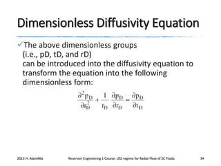
![Diffusivity Constant
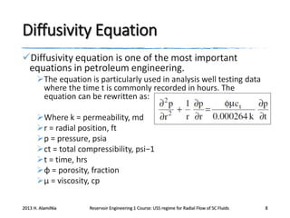
The term [0.000264 k/φμct] is called the diffusivity
constant and is denoted by the symbol η, or:
The diffusivity equation can then be written in a
more convenient form as:
2013 H. AlamiNia
Reservoir Engineering 1 Course: USS regime for Radial Flow of SC Fluids
10](https://image.slidesharecdn.com/q913-re1-20w3-20lec-209-131101231219-phpapp01/85/Q913-re1-w3-lec-9-10-320.jpg)


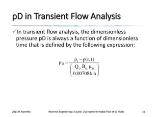
![Dimensionless Pressure
It is obvious that the right hand side of the above
equation has no units (i.e., dimensionless) and,
accordingly, the left-hand side must be
dimensionless.
Since the left-hand side is dimensionless, and (pe −
pwf) has the units of psi, it follows that the term
[Qo Bo μo/ (0.00708kh)] has units of pressure.
2013 H. AlamiNia
Reservoir Engineering 1 Course: USS regime for Radial Flow of SC Fluids
30](https://image.slidesharecdn.com/q913-re1-20w3-20lec-209-131101231219-phpapp01/85/Q913-re1-w3-lec-9-30-320.jpg)


This document provides an overview of unsteady-state flow and the diffusivity equation, which is used to model pressure changes over time in reservoirs. It discusses the assumptions and solutions of the diffusivity equation, including the Ei-function and dimensionless pressure drop solutions. The constant-terminal pressure and constant-terminal rate solutions are examined. Graphs demonstrate how pressure profiles change over different times based on these solutions. The document also explores using dimensionless variables to simplify analyses of unsteady-state flow regimes.