Downloaded 74 times
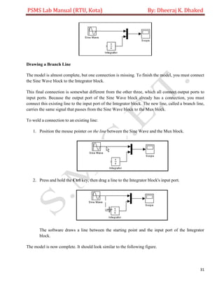
![PSMS Lab Manual (RTU, Kota) By: Dheeraj K. Dhaked
12
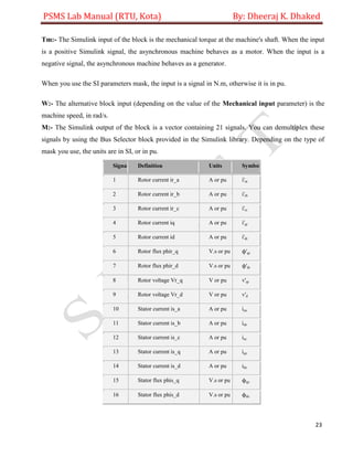
ifn 1087 A
ifd [695.64, 774.7, 917.5, 1001.6, 1082.2, 1175.9, 1293.6, 1430.2, 1583.7] A
Vt [9660, 10623, 12243, 13063, 13757, 14437, 15180, 15890, 16567] V
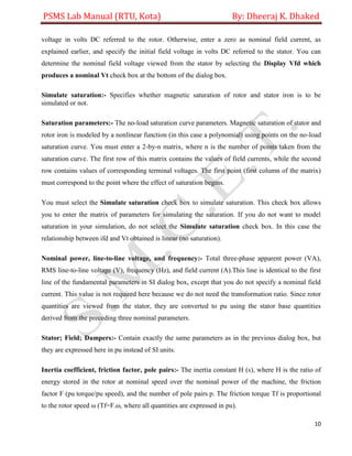
Sample time (-1 for inherited)
Specifies the sample time used by the block. To inherit the sample time specified in the
Powergui block, set this parameter to -1.
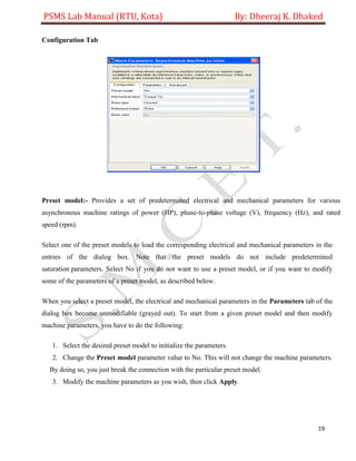
Inputs and Outputs:- The units of inputs and outputs vary according to which dialog box was used
to enter the block parameters. If the fundamental parameters in SI units is used, the inputs and
outputs are in SI units (except for dw in the vector of internal variables, which is always in pu, and
angle Θ, which is always in rad). Otherwise, the inputs and outputs are in pu.
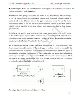
Pm:- The first Simulink input is the mechanical power at the machine's shaft. In generating mode,
this input can be a positive constant or function or the output of a prime mover block (see the
Hydraulic Turbine and Governor or Steam Turbine and Governor blocks). In motoring mode, this
input is usually a negative constant or function.](https://image.slidesharecdn.com/psmslabmanual-170809085023/85/Psms-lab-manual-12-320.jpg)
![PSMS Lab Manual (RTU, Kota) By: Dheeraj K. Dhaked
36
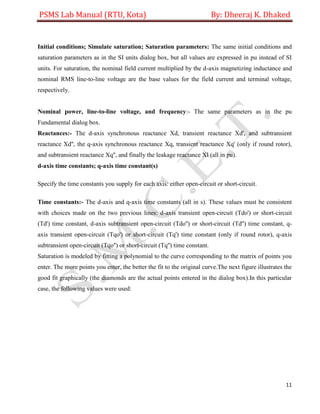
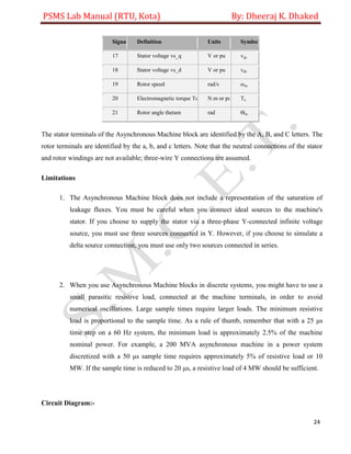
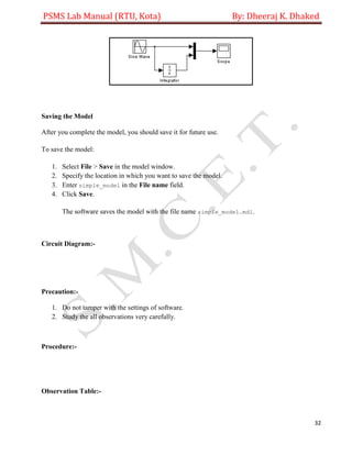
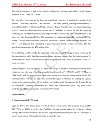
Make sure that the operation mode is set to “UPFC (Power Flow Control)”. The reference active and
reactive powers are specified in the last two lines of the GUI menu. Initially, Pref= +8.7
pu/100MVA (+870 MW) and Qref=-0.6 pu/100MVA (-60 Mvar). At t=0.25 sec Pref is changed to
+10 pu (+1000MW). Then, at t=0.5 sec, Qref is changed to +0.7 pu (+70 Mvar). The reference
voltage of the shunt converter (specified in the 2nd line of the GUI) will be kept constant at Vref=1
pu during the whole simulation (Step Time=0.3*100> Simulation stop time (0.8 sec). When the
UPFC is in power control mode, the changes in STATCOM reference reactive power and in SSSC
injected voltage (specified respectively in 1st and 3rd line of the GUI) as are not used.
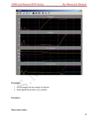
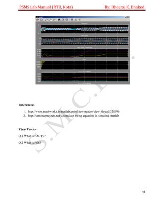
Run the simulation for 0.8 sec. Open the “Show Scopes” subsystem. Observe on traces 1 and 2 of
the UPFC scope the variations of P and Q. After a transient period lasting approximately 0.15 sec,
the steady state is reached (P=+8.7 pu; Q=-0.6 pu). Then P and Q are ramped to the new settings
(P=+10 pu Q=+0.7 pu). Observe on traces 3 and 4 the resulting changes in P Q on the three
transmission lines. The performance of the shunt and series converters can be observed respectively
on the STATCOM and SSSC scopes. If you zoom on the first trace of the STATCOM scope, you
can observe the 48-step voltage waveform Vs generated on the secondary side of the shunt converter
transformers (yellow trace) superimposed with the primary voltage Vp (magenta) and the primary
current Ip (cyan). The dc bus voltage (trace 2) varies in the 19kV-21kV range. If you zoom on the
first trace of the SSSC scope, you can observe the injected voltage waveforms Vinj measured
between buses B1 and B2.
2. Var control in STATCOM mode
In the GUI block menu, change the operation mode to “STATCOM (Var Control)”. Make sure that
the STATCOM references values (1st line of parameters, [T1 T2 Q1 Q2]) are set to [0.3 0.5 +0.8 -
0.8 ]. In this mode, the STATCOM is operated as a variable source of reactive power. Initially, Q is
set to zero, then at T1=0.3 sec Q is increased to +0.8 pu (STATCOM absorbing reactive power) and
at T2=0.5 sec, Q is reversed to -0.8 pu (STATCOM generating reactive power).
Run the simulation and observe on the STATCOM scope the dynamic response of the STATCOM.
Zoom on the first trace around t=0.5 sec when Q is changed from +0.8 pu to -0.8 pu. When Q=+0.8
pu, the current flowing into the STATCOM (cyan trace) is lagging voltage (magenta trace),
indicating that STATCOM is absorbing reactive power. When Qref is changed from +0.8 to -0.8, the](https://image.slidesharecdn.com/psmslabmanual-170809085023/85/Psms-lab-manual-36-320.jpg)
![PSMS Lab Manual (RTU, Kota) By: Dheeraj K. Dhaked
37
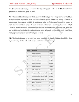
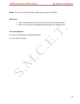
current phase shift with respect to voltage changes from 90 degrees lagging to 90 degrees leading
within one cycle. This control of reactive power is obtained by varying the magnitude of the
secondary voltage Vs generated by the shunt converter while keeping it in phase with the bus B1
voltage Vp. This change of Vs magnitude is performed by controlling the dc bus voltage. When Q is
changing from +0.8 pu to -0.8 pu, Vdc (trace 3) increases from 17.5 kV to 21 kV.
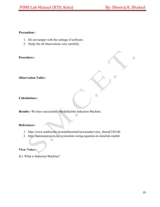
3. Series voltage injection in SSSC mode
In the GUI block menu change the operation mode to “SSSC (Voltage injection)”. Make sure that
the SSSC references values (3rd line of parameters) [Vinj_Initial Vinj_Final StepTime] ) are set to
[0.0 0.08 0.3 ]. The initial voltage is set to 0 pu, then at t=0.3 sec it will be ramped to 0.8 pu.
Run the simulation and observe on the SSSC scope the impact of injected voltage on P and Q
flowing in the 3 transmission lines. Contrary to the UPFC mode, in SSCC mode the series inverter
operates with a constant conduction angle (Sigma= 172.5 degrees). The magnitude of the injected
voltage is controlled by varying the dc voltage which is proportional to Vinj (3rd trace). Also,
observe the waveforms of injected voltages (1st trace) and currents flowing through the SSSC (2nd
trace). Voltages and currents stay in quadrature so that the SSSC operates as a variable inductance or
capacitance.
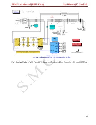
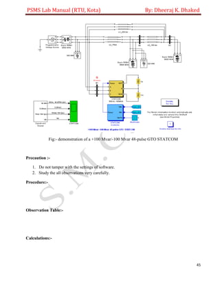
Circuit Diagram:-](https://image.slidesharecdn.com/psmslabmanual-170809085023/85/Psms-lab-manual-37-320.jpg)

This document is a lab manual for a Power System Modeling and Simulation course. It contains instructions for 6 experiments involving modeling synchronous machines, induction machines, and FACTS devices in MATLAB/Simulink. The first experiment provides the swing equation that governs rotor motion of a synchronous machine and guides students in simulating it in Simulink. Subsequent experiments instruct students on modeling synchronous machines, induction machines, and implementing various FACTS controllers for a single-machine infinite-bus system.