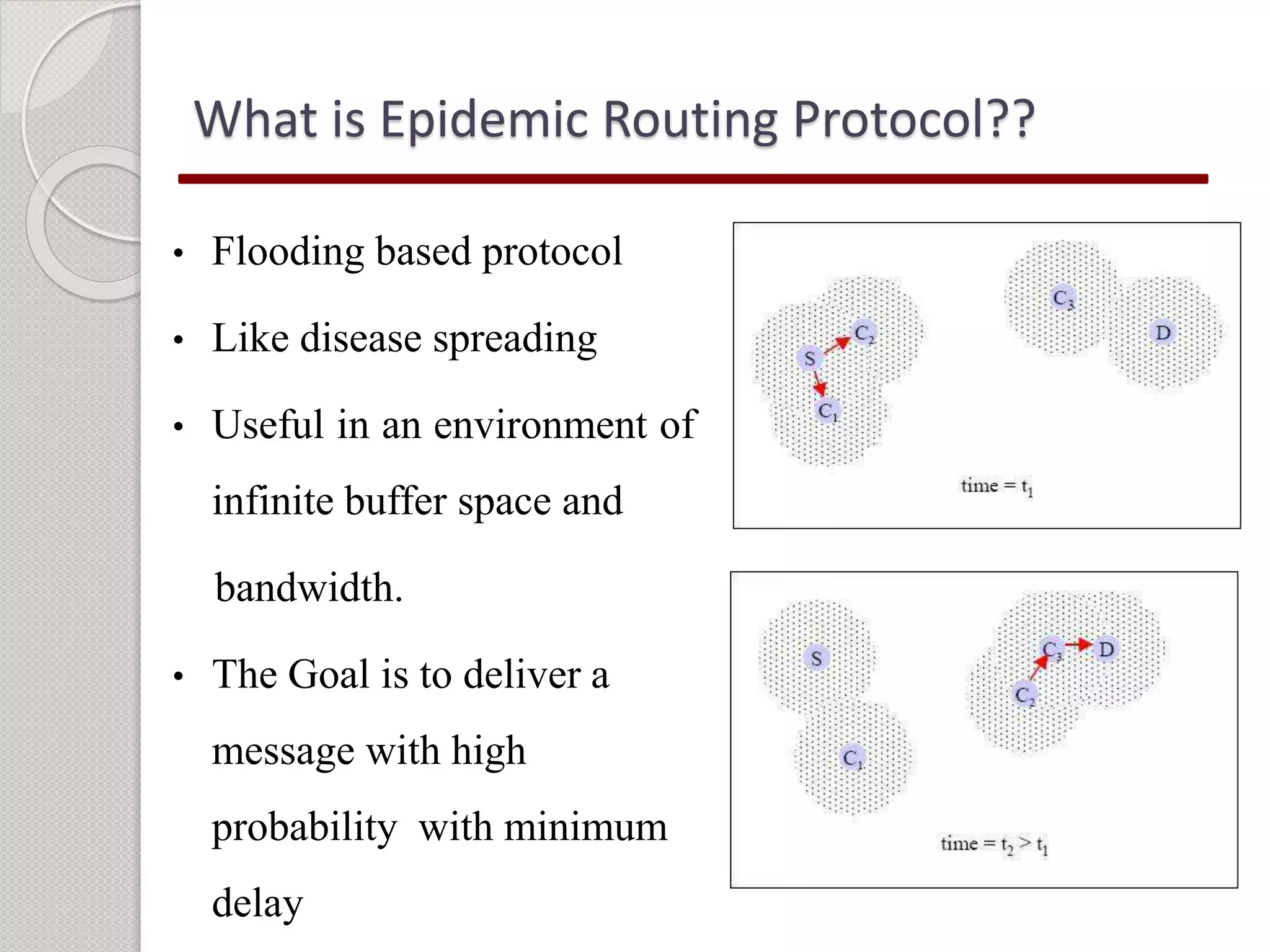
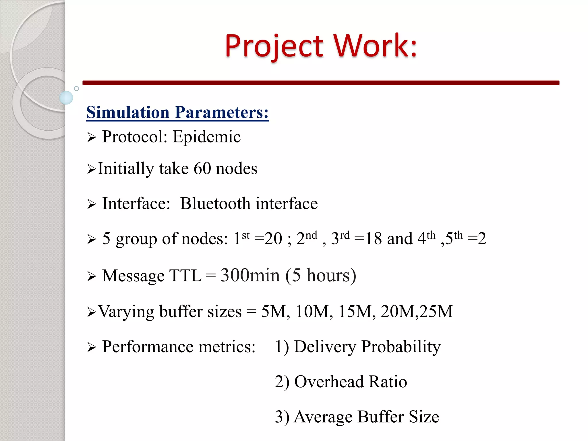
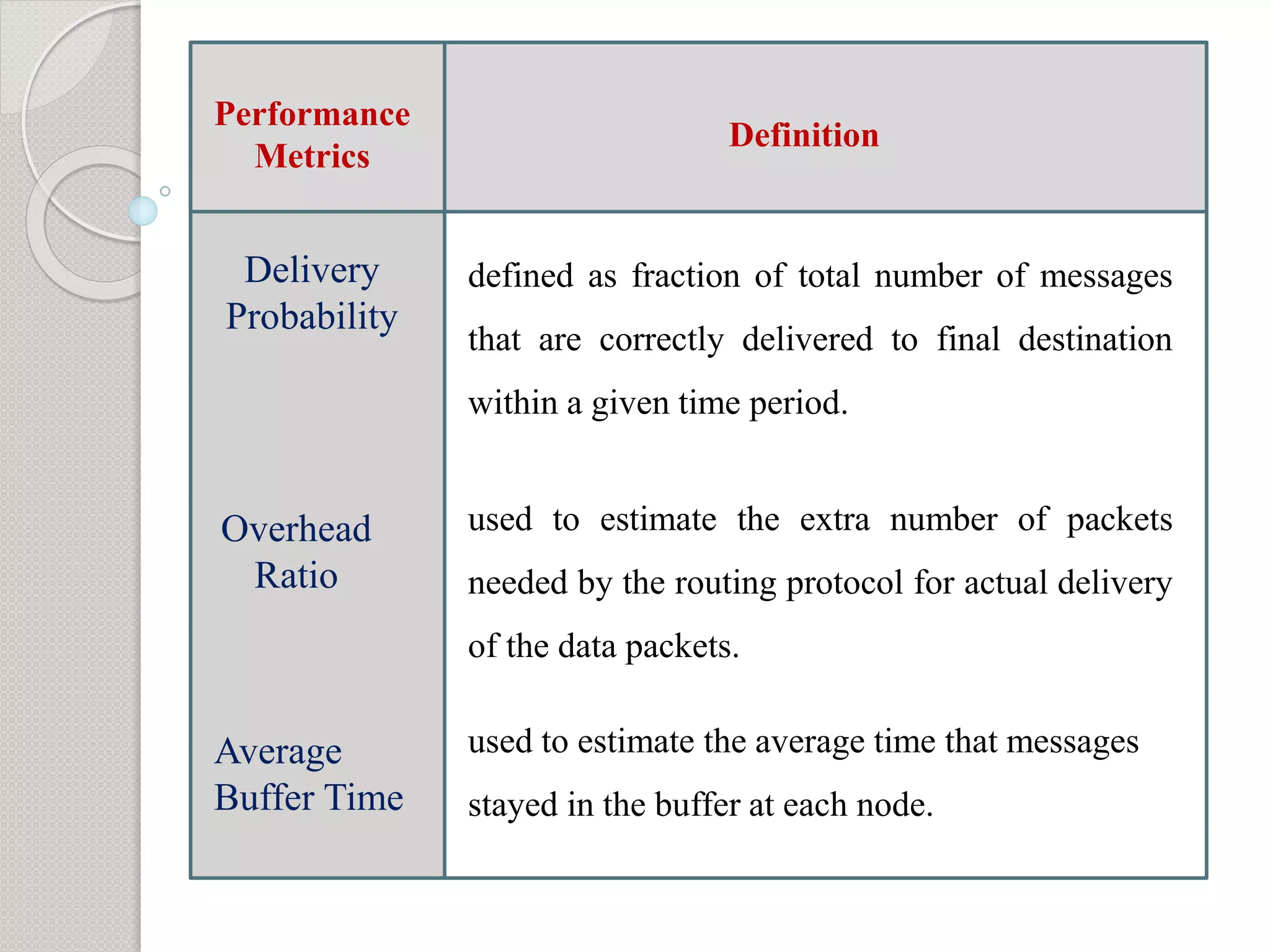
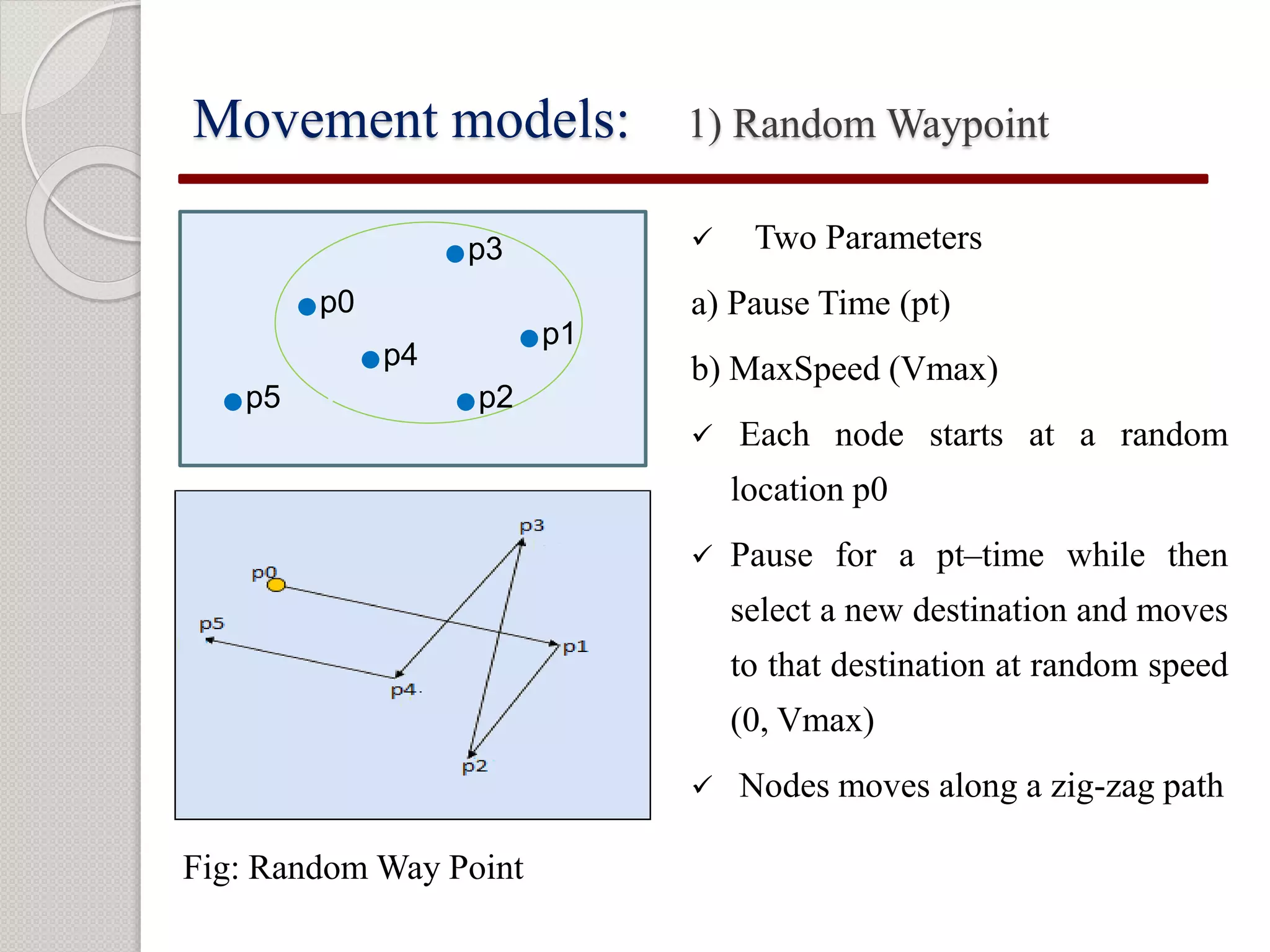
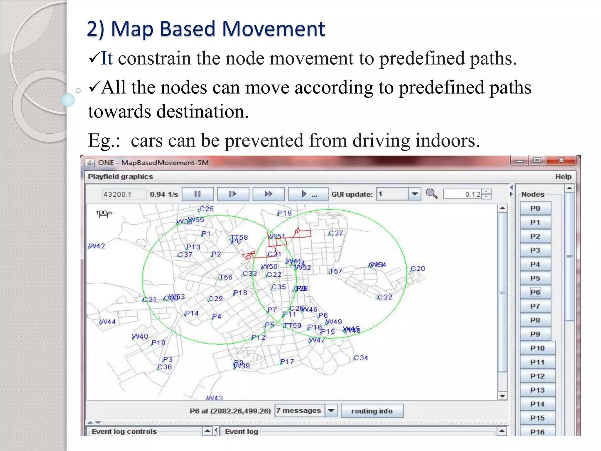
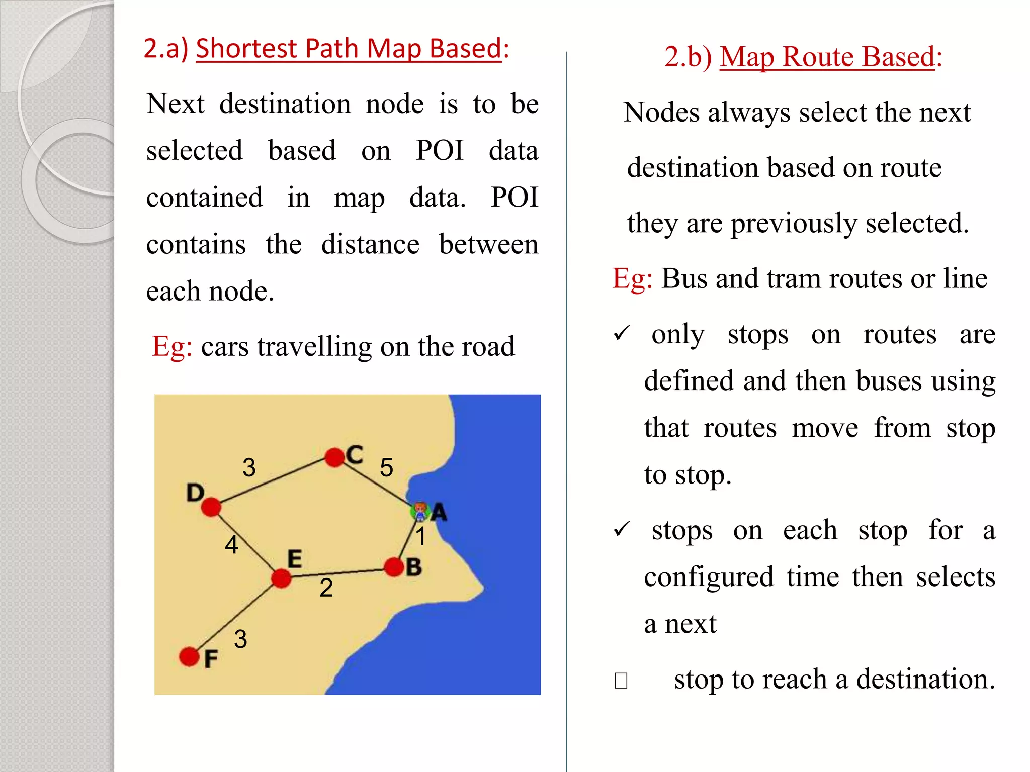
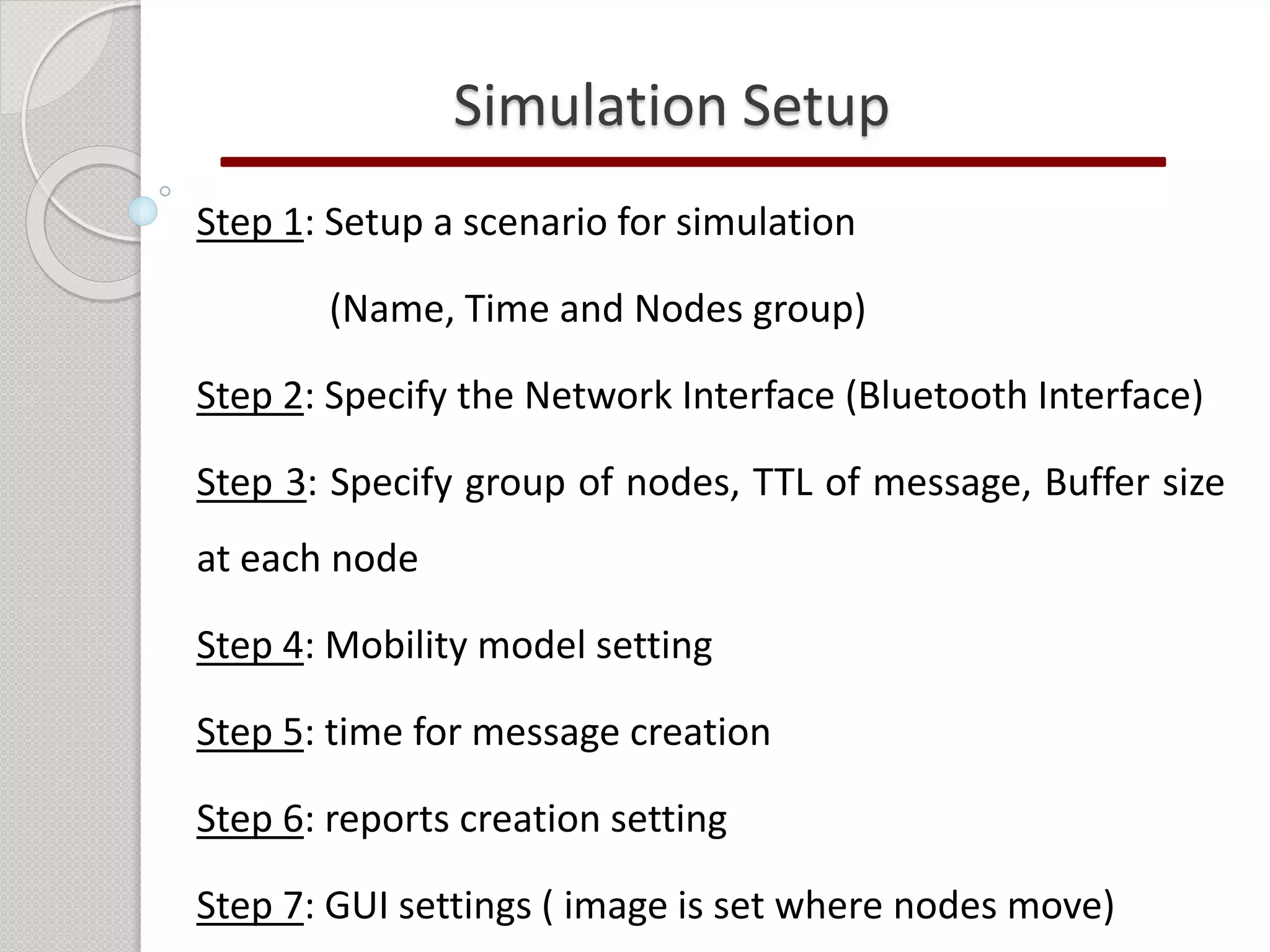
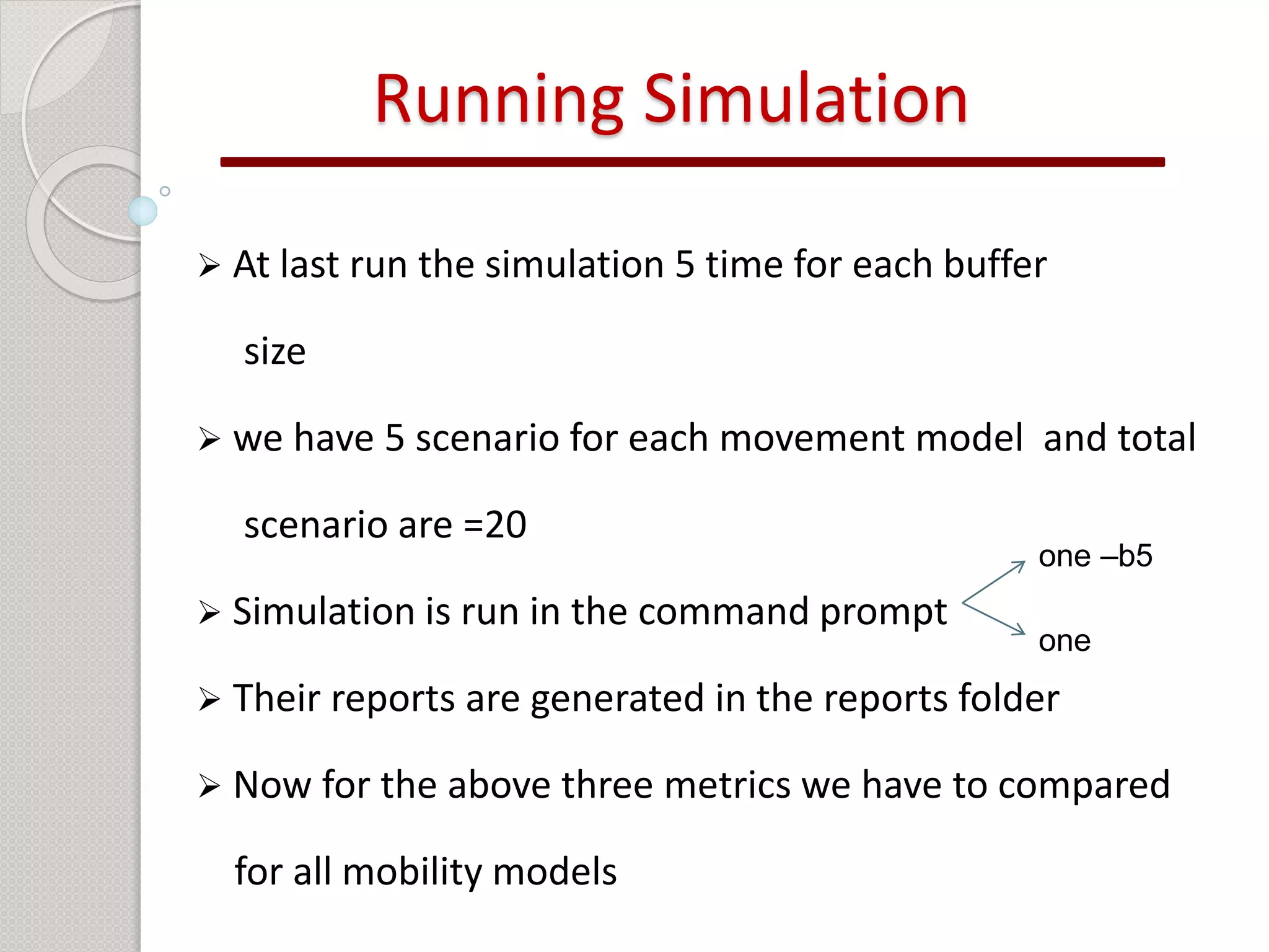
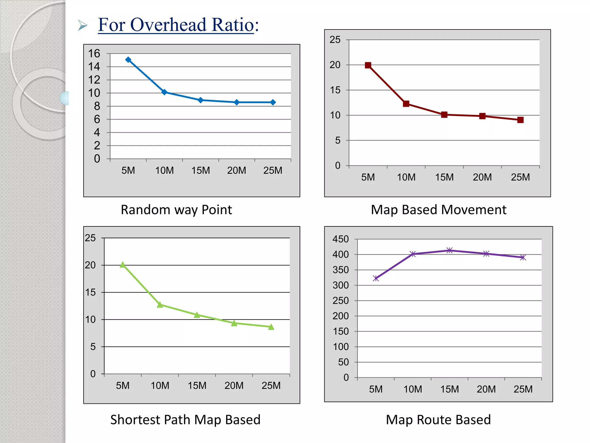
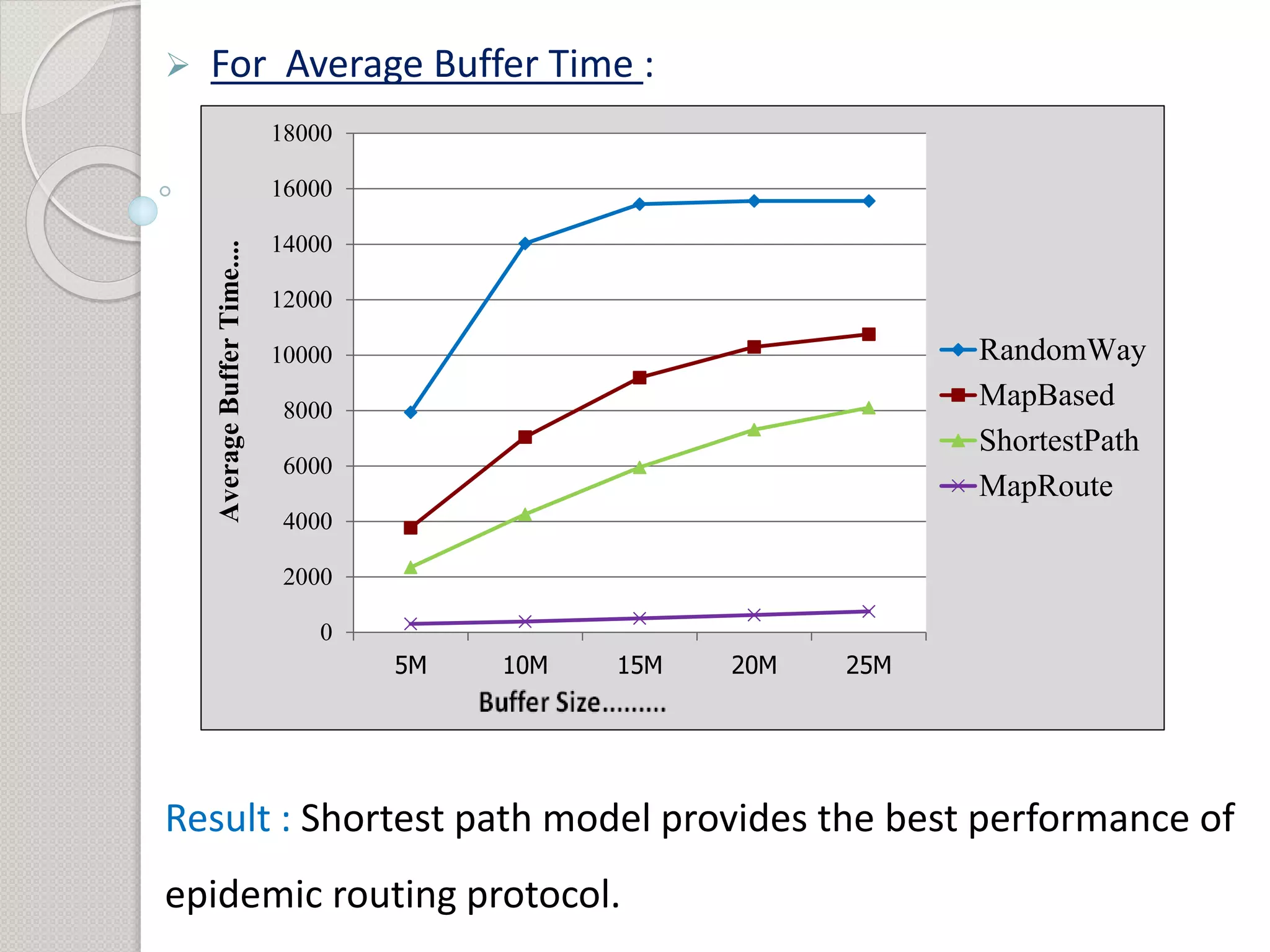
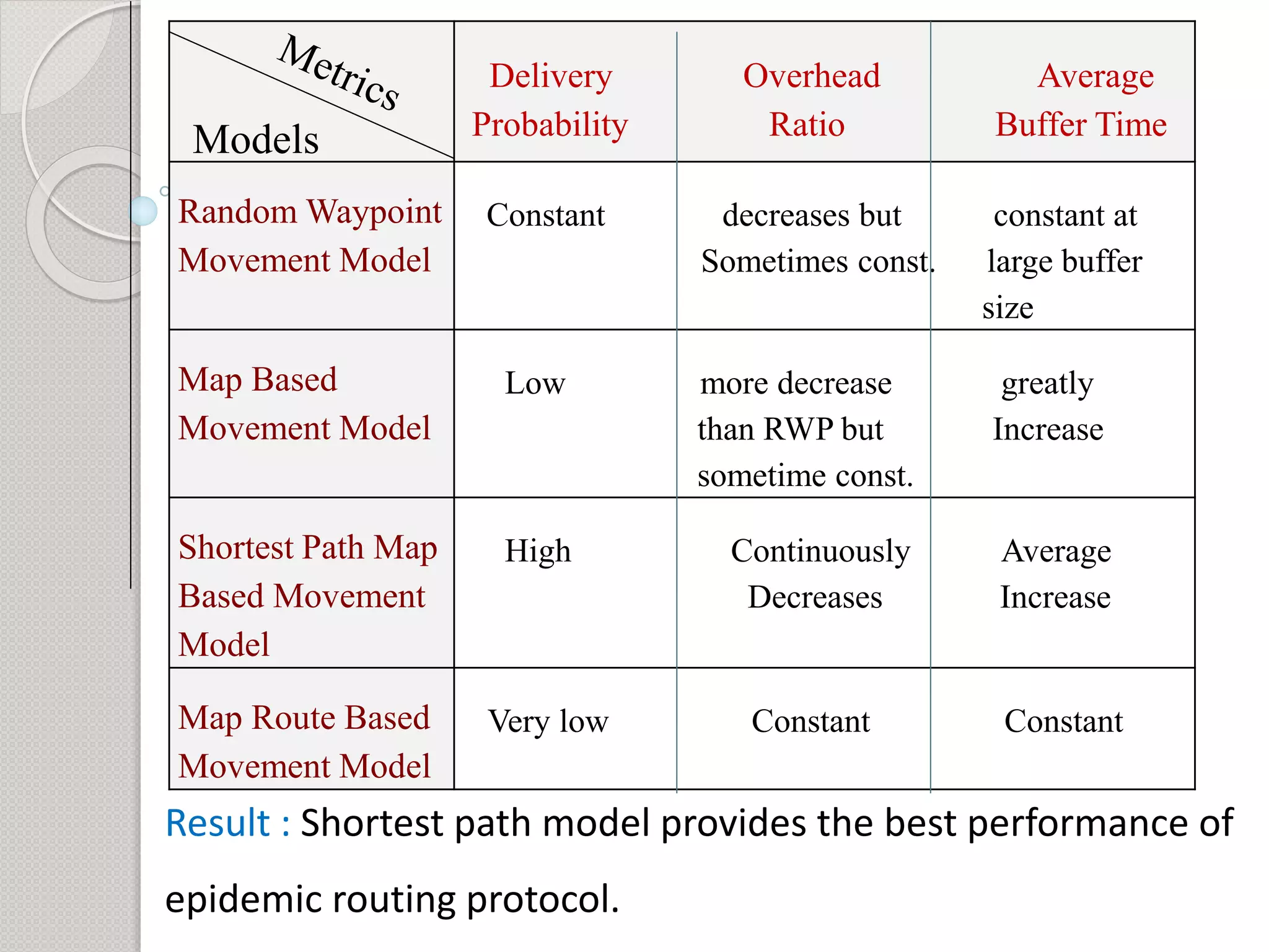
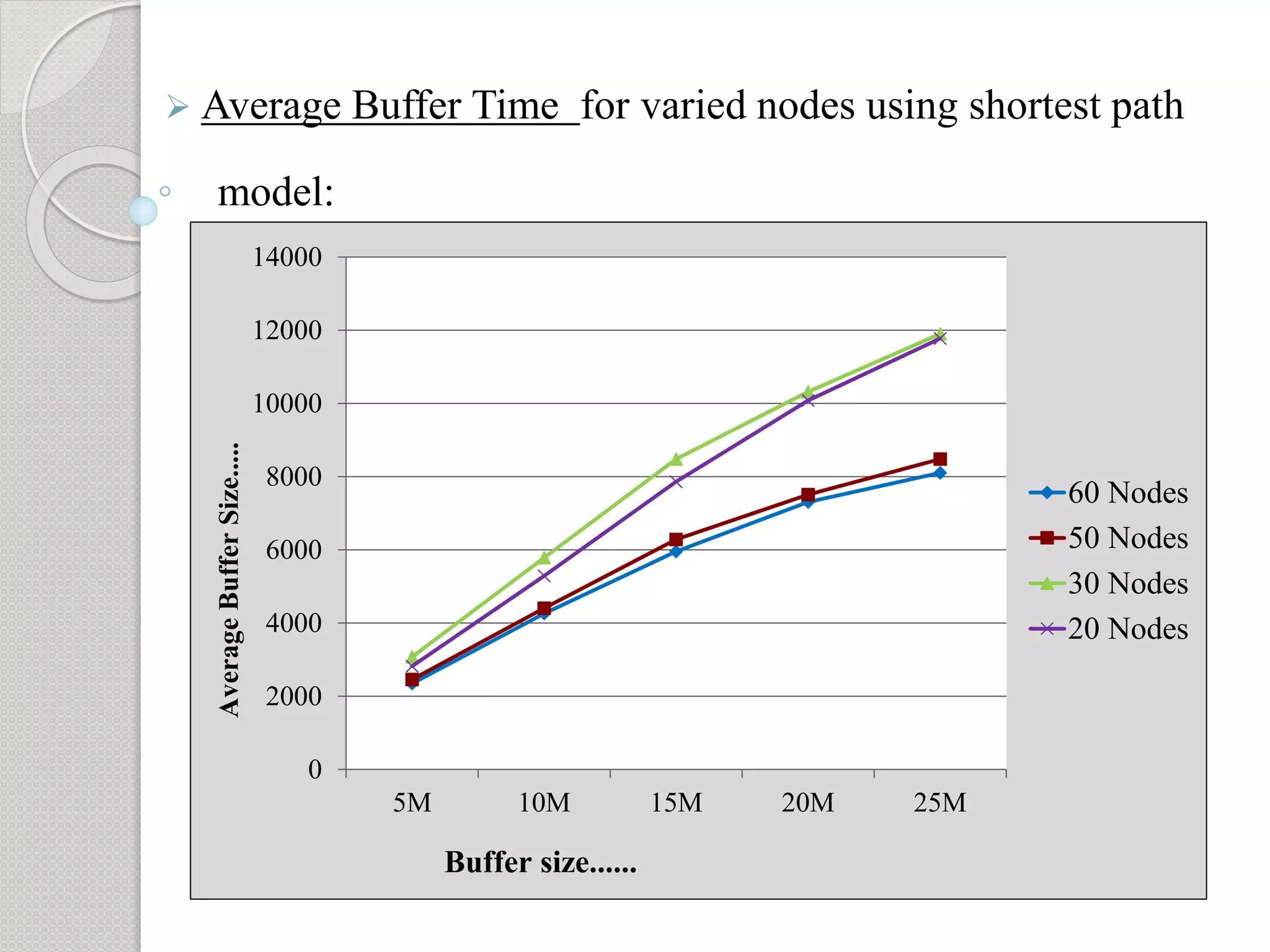
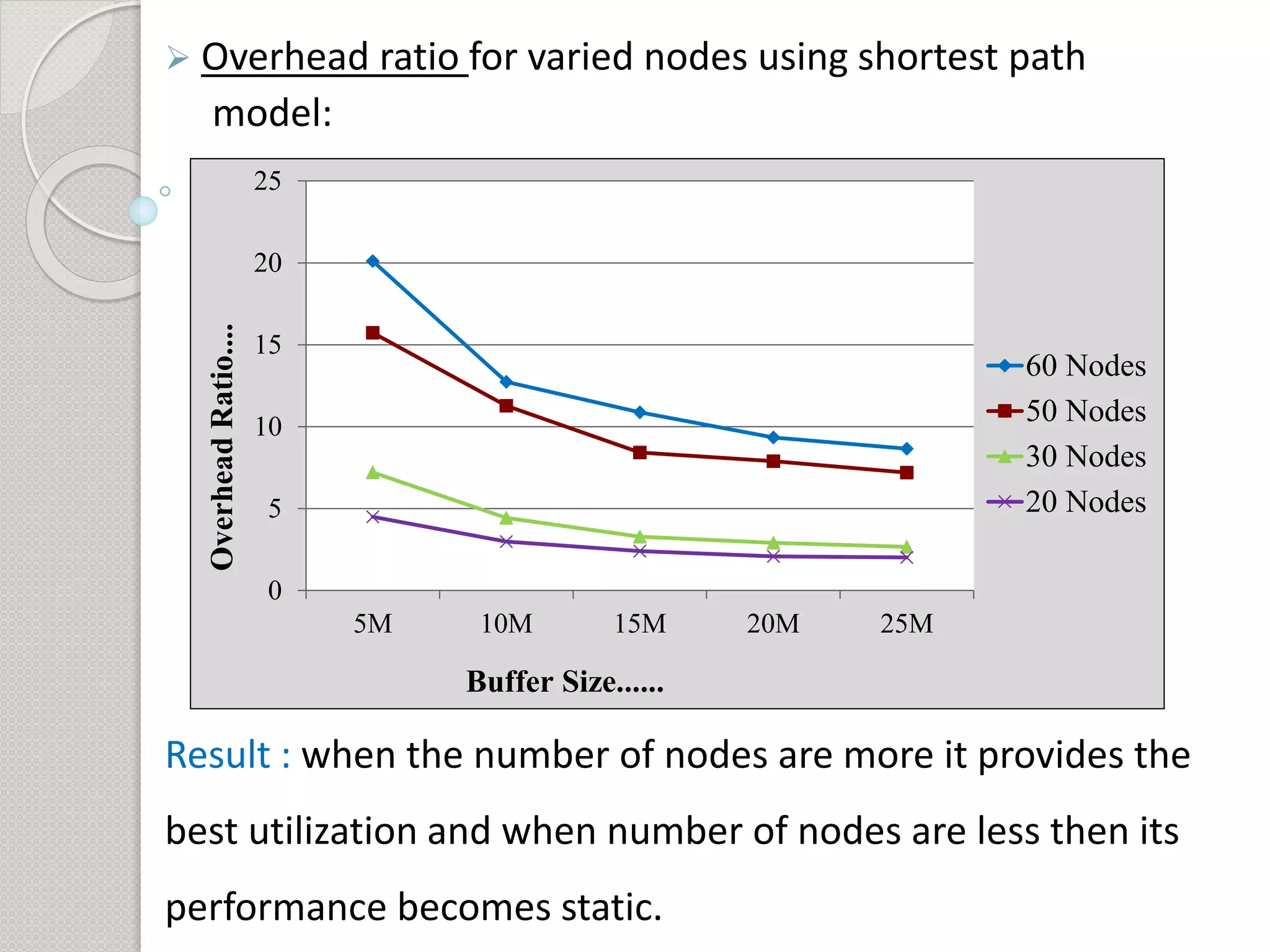
This document summarizes a project seminar presentation on analyzing the performance of the epidemic routing protocol in delay tolerant networks under different mobility models. The key points are: 1) The objective is to evaluate the epidemic routing protocol's delivery probability, overhead ratio, and average buffer time when varying the buffer size and under different mobility models including random waypoint, map-based, shortest path, and map route models. 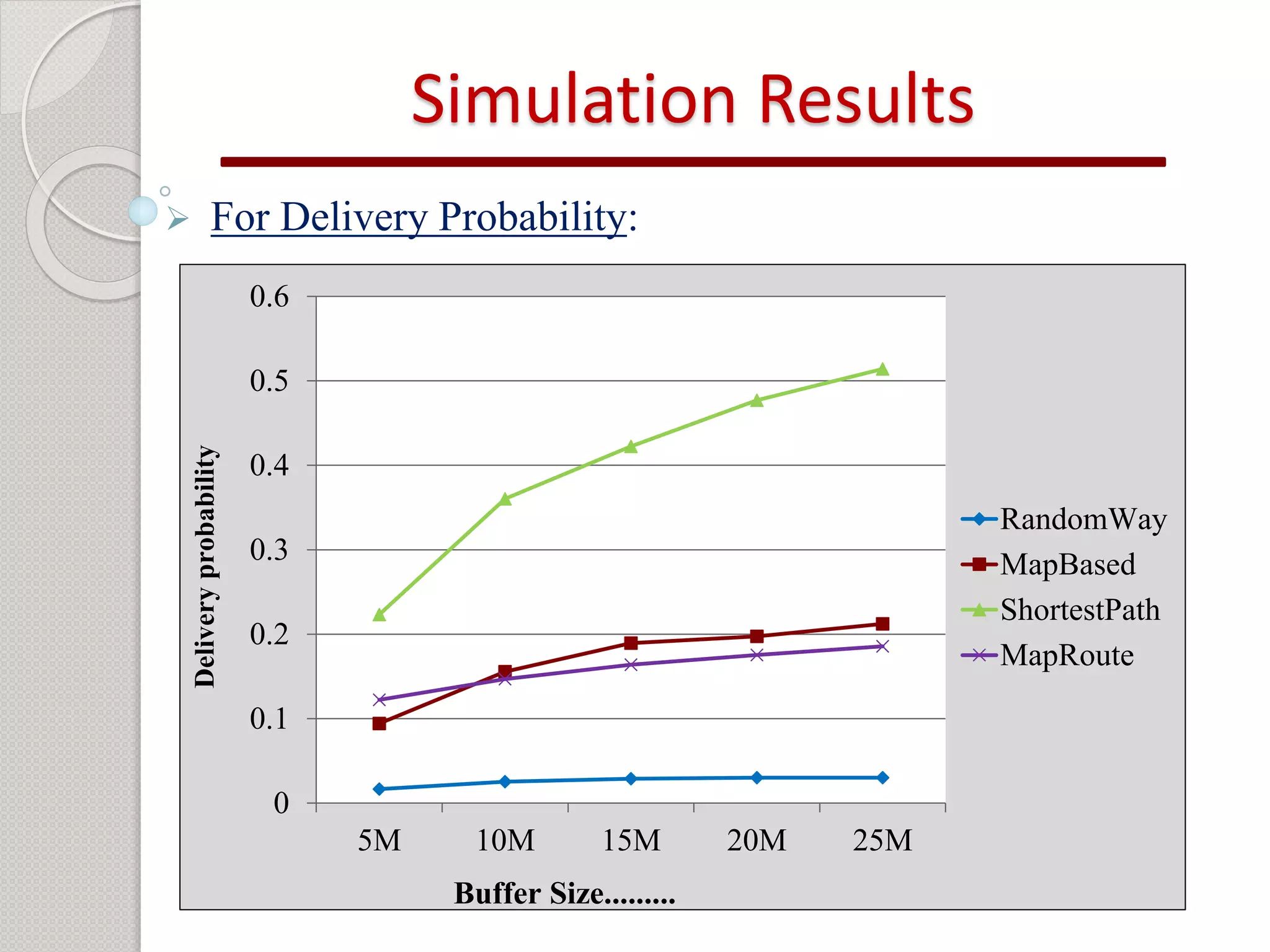2) Simulation results show that the shortest path mobility model provides the best performance for the epidemic routing protocol in terms of high delivery probability, low overhead ratio, and efficient buffer usage. 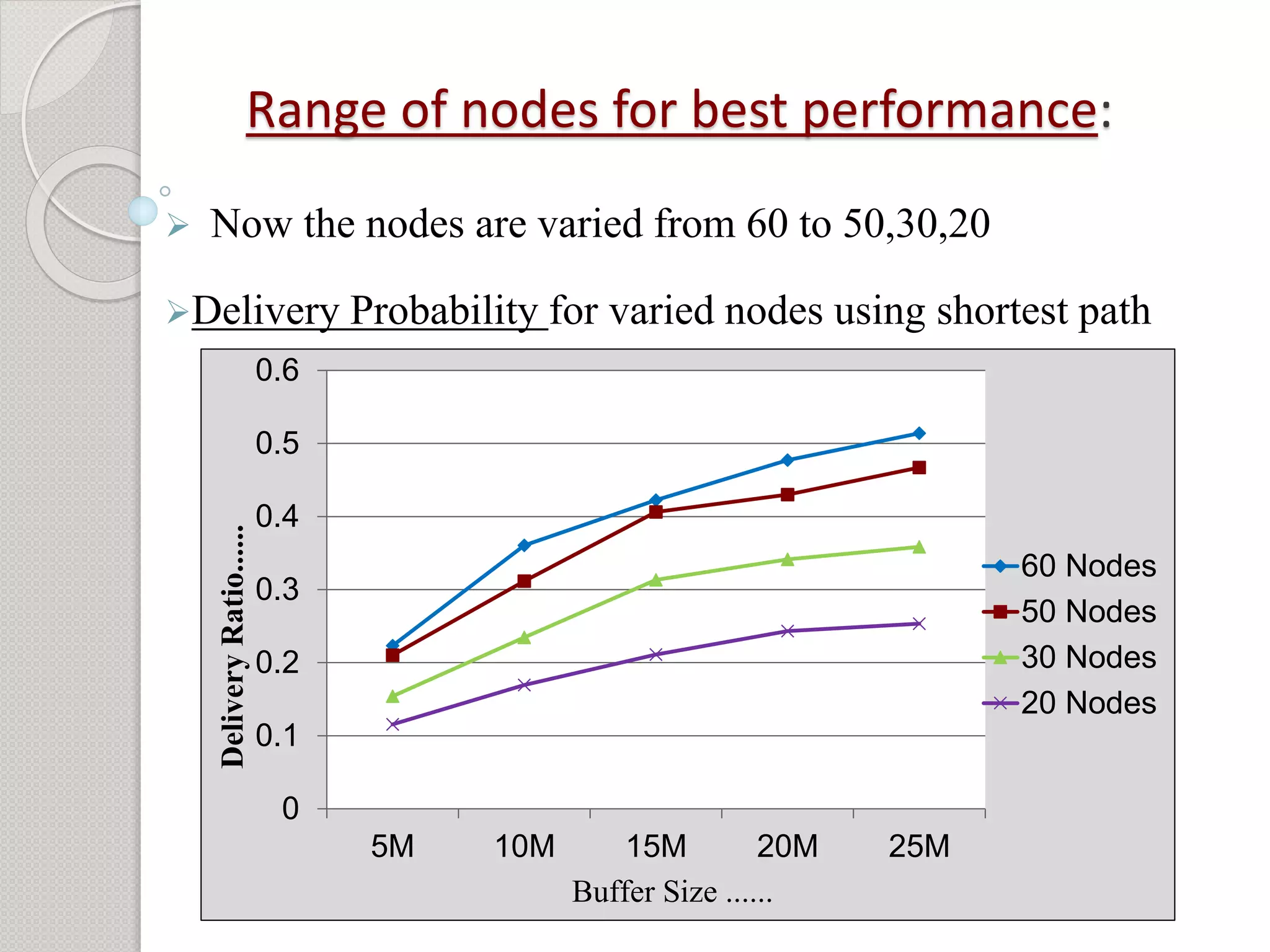3) Additional analysis varying the number of nodes found that performance is best when more nodes are present and becomes static with

1. Project Seminar
On
“Performance Analysis of
Epidemic Routing Protocol in DTN”
Presented by:
Jashanpreet pal Kaur
M.Tech- CE

2. Why DTN??????
Adhoc networks
1)The protocols first establish
a end to end path between
source and destination to
communicate.
2)Delays are more
DTN
1)Follow Store & Forward
approach
• Intermittent connectivity
• Opportunistic N/w’s
2)Less delays (delay tolerate
3)Consist of variousprotocols:
Epidemic, PRoHET, Spray
&wait, direct delivery, First
contact

3. What is Epidemic Routing Protocol??
• Flooding based protocol
• Like disease spreading
• Useful in an environment of
infinite buffer space and
bandwidth.
• The Goal is to deliver a
message with high
probability with minimum
delay

4. PROJECT OBJECTIVE
• The main objective is to check that for which mobility
models among the Random waypoint, Map based
mobility , Shortest Path Movement, and Map Route
based movement the Epidemic protocol performs best
when buffer size at each node is varied.
• At what range of nodes its performance is best or static.

5. Methodology Used
• ONE –Opportunistic Networking Environment Simulator
( Latest version 1.4.1)
• Java Based Simulator for research in DTN’s
• Runs on Linux,Windows or any platform that supporting
a Java
• Users can simulate different scenarios in easily and flexible
manner for routing protocols based on mobility models.

6. Continue……
• It combines Movement models, Routing simulations,
Visualization and Reports into one program.

7. Project Work:
Simulation Parameters:
 Protocol: Epidemic
Initially take 60 nodes
 Interface: Bluetooth interface
 5 group of nodes: 1st =20 ; 2nd , 3rd =18 and 4th ,5th =2
 Message TTL = 300min (5 hours)
Varying buffer sizes = 5M, 10M, 15M, 20M,25M
 Performance metrics: 1) Delivery Probability
2) Overhead Ratio
3) Average Buffer Size

8. Performance
Metrics
Definition
Delivery
Probability
Overhead
Ratio
Average
Buffer Time
defined as fraction of total number of messages
that are correctly delivered to final destination
within a given time period.
used to estimate the extra number of packets
needed by the routing protocol for actual delivery
of the data packets.
used to estimate the average time that messages
stayed in the buffer at each node.

9. Movement models: 1) Random Waypoint
Fig: RandomWay Point
 Two Parameters
a) Pause Time (pt)
b) MaxSpeed (Vmax)
 Each node starts at a random
location p0
 Pause for a pt–time while then
select a new destination and moves
to that destination at random speed
(0, Vmax)
 Nodes moves along a zig-zag path
p0
p3
p1
p2
p4
p5

10. Continue………

11. 2) Map Based Movement
It constrain the node movement to predefined paths.
All the nodes can move according to predefined paths
towards destination.
Eg.: cars can be prevented from driving indoors.

12. 2.a) Shortest Path Map Based:
Next destination node is to be
selected based on POI data
contained in map data. POI
contains the distance between
each node.
Eg: cars travelling on the road
2.b) Map Route Based:
Nodes always select the next
destination based on route
they are previously selected.
Eg: Bus and tram routes or line
 only stops on routes are
defined and then buses using
that routes move from stop
to stop.
 stops on each stop for a
configured time then selects
a next
stop to reach a destination.
1
5
1
3
4
2
3

13. Simulation Setup
Step 1: Setup a scenario for simulation
(Name, Time and Nodes group)
Step 2: Specify the Network Interface (Bluetooth Interface)
Step 3: Specify group of nodes, TTL of message, Buffer size
at each node
Step 4: Mobility model setting
Step 5: time for message creation
Step 6: reports creation setting
Step 7: GUI settings ( image is set where nodes move)

14. Running Simulation
 At last run the simulation 5 time for each buffer
size
 we have 5 scenario for each movement model and total
scenario are =20
 Simulation is run in the command prompt
 Their reports are generated in the reports folder
 Now for the above three metrics we have to compared
for all mobility models
one –b5
one

15. Simulation Results
 For Delivery Probability:
0.6
0.5
0.4
0.3
0.2
0.1
0
5M 10M 15M 20M 25M
RandomWay
MapBased
ShortestPath
MapRoute
Buffer Size.........
Delivery probability

16.  For Overhead Ratio:
25
20
15
10
5
Random way Point Map Based Movement
450
400
350
300
250
200
150
100
50
Shortest Path Map Based Map Route Based
16
14
12
10
8
6
4
2
0
5M 10M 15M 20M 25M
0
5M 10M 15M 20M 25M
25
20
15
10
5
0
5M 10M 15M 20M 25M
0
5M 10M 15M 20M 25M

17.  For Average Buffer Time :
18000
16000
14000
12000
10000
8000
6000
4000
2000
0
5M 10M 15M 20M 25M
RandomWay
MapBased
ShortestPath
MapRoute
Average Buffer Time....
Result : Shortest path model provides the best performance of
epidemic routing protocol.

18. Delivery Overhead Average
Probability Ratio Buffer Time
Models
Random Waypoint
Movement Model
Constant decreases but constant at
Sometimes const. large buffer
size
Map Based
Movement Model
Low more decrease greatly
than RWP but Increase
sometime const.
Shortest Path Map
Based Movement
Model
High Continuously Average
Decreases Increase
Map Route Based
Movement Model
Very low Constant Constant
Result : Shortest path model provides the best performance of
epidemic routing protocol.

19. Range of nodes for best performance:
 Now the nodes are varied from 60 to 50,30,20
Delivery Probability for varied nodes using shortest path
0.6
model:
0.5
0.4
0.3
0.2
0.1
0
5M 10M 15M 20M 25M
60 Nodes
50 Nodes
30 Nodes
20 Nodes
Delivery Ratio......
Buffer Size ......

20.  Average Buffer Time for varied nodes using shortest path
model:
14000
12000
10000
8000
6000
4000
2000
0
5M 10M 15M 20M 25M
60 Nodes
50 Nodes
30 Nodes
20 Nodes
Buffer size......
Average Buffer Size.....

21.  Overhead ratio for varied nodes using shortest path
model:
25
20
15
10
5
0
5M 10M 15M 20M 25M
60 Nodes
50 Nodes
30 Nodes
20 Nodes
Overhead Ratio....
Buffer Size......
Result : when the number of nodes are more it provides the
best utilization and when number of nodes are less then its
performance becomes static.

22. Conclusion
The analysis of scenarios concludes that the shortest path
map based mobility model is best among all for routing
using epidemic routing protocol. Then after varying the
number of nodes concludes that this model provides the
best delivery ratio and less overheads when number of
nodes is more and static performance when number of
nodes are too less.

23. Future Scope
There are two main problems in the epidemic routing
protocol. It comsumes a lot of resources and unauthorized
access to the messages. Then it is further interesting to see
the malicious node effects to recover the messages from
them and for decreasing the resource consumption instead
of using FIFO strategy, we can any other strategy or
removing the messages from the buffer that has already
forwarded. The Quota sampling is used instead of using the
flooding strategy.

24. References
[1] Professor Jorg Ott of Helinski University of Technology: “A Tutorial paper on the
Opportunistic Networking Environment Simulator” presented in May 29, 2008
[2] Paritosh Puri, M.P Singh: “A Survey paper on Delay Tolerant Networking”presented in
2013.
[3] Harminder Singh Bindra and A. L. Sangal:“ The Performance comparison of the
RAPID,
Epidemic, PRoHET routing protocols in DTN ” presented in the April 2, 2012.
[4] Anders Lindgreny, Avri Doria, Olov Schelen: “The Probabilistic Routing in case of DTN
Intermittently Connected Networks” presented in December 2002.
[5] Neena V V, V Mary Anita Rajam: “Performance Analysis of Epidemic Routing Protocol
for
Opportunistic Networks in Different Mobility Patterns ” presentesd in Jan. 09, 2013.
[6] Forrest Warthman : “A Tutorial Delay tolerant networks” presented in May 3, 2003.
[7] Sushant Jain, Kevin Fall, Rabin Patra: “Routing in DTN” presented in Aug 4, 2008.

25. Thank You