


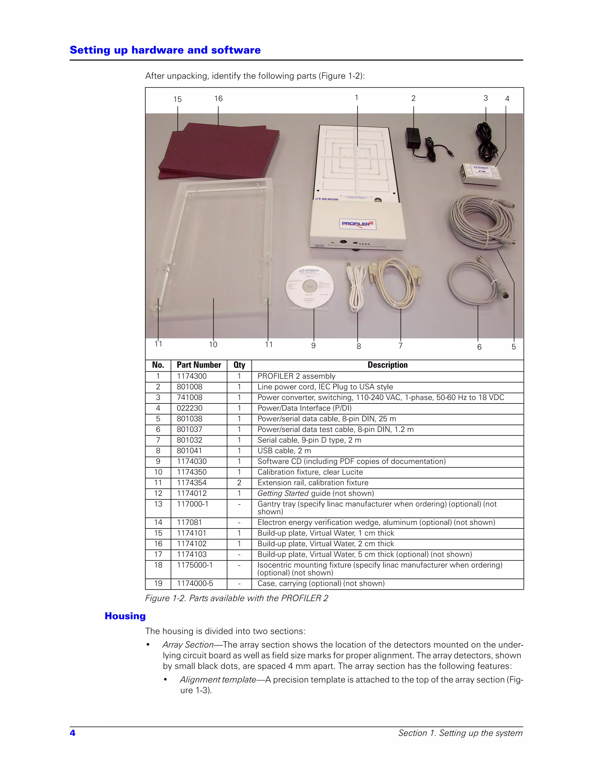
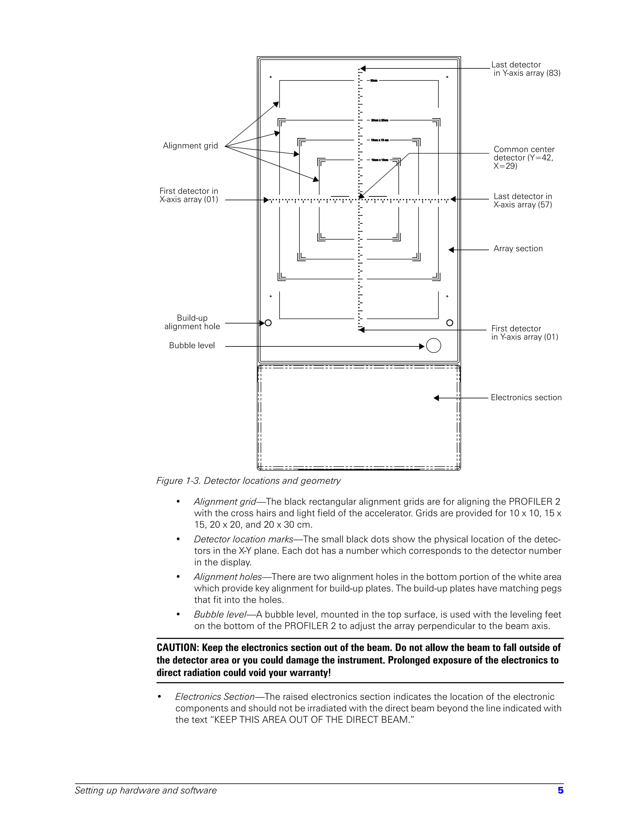
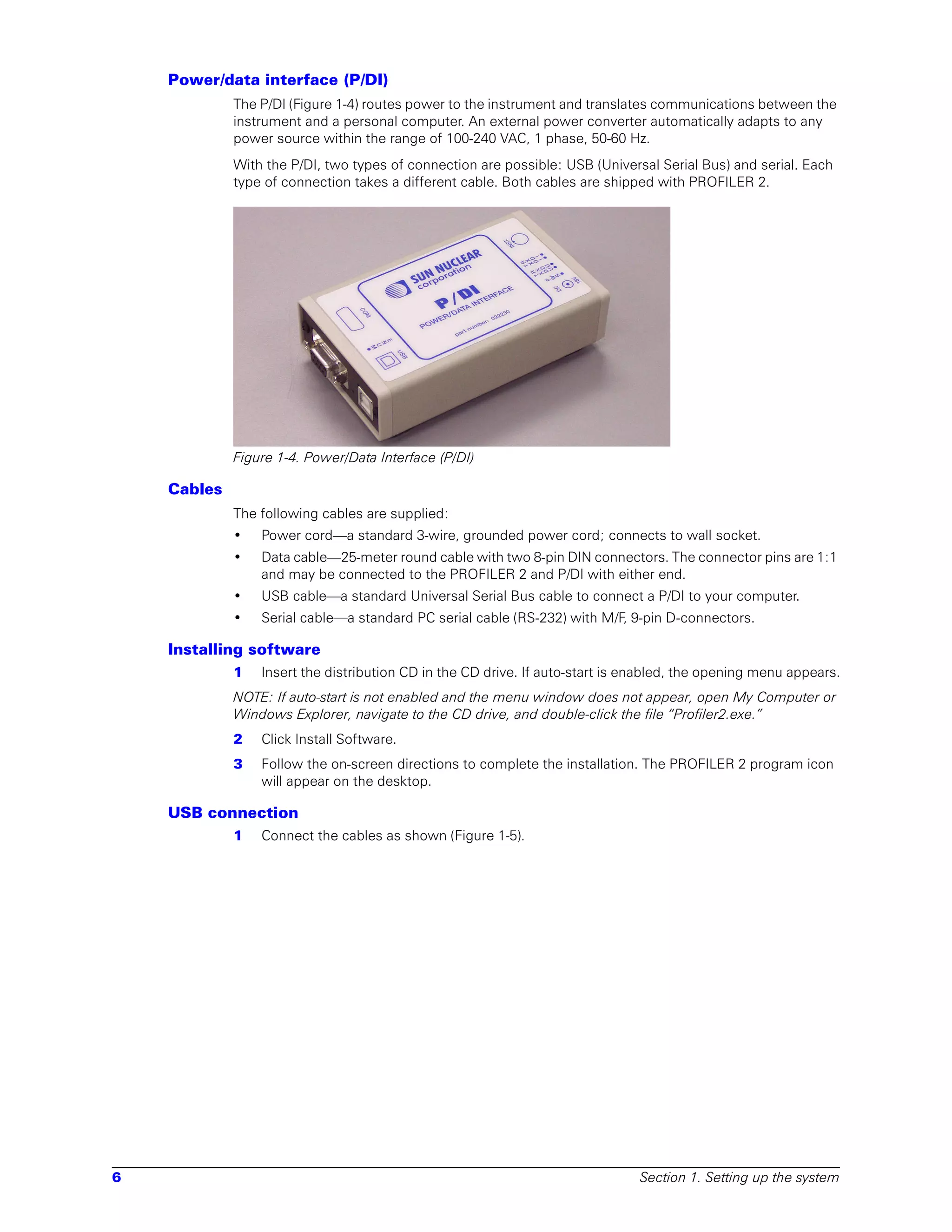
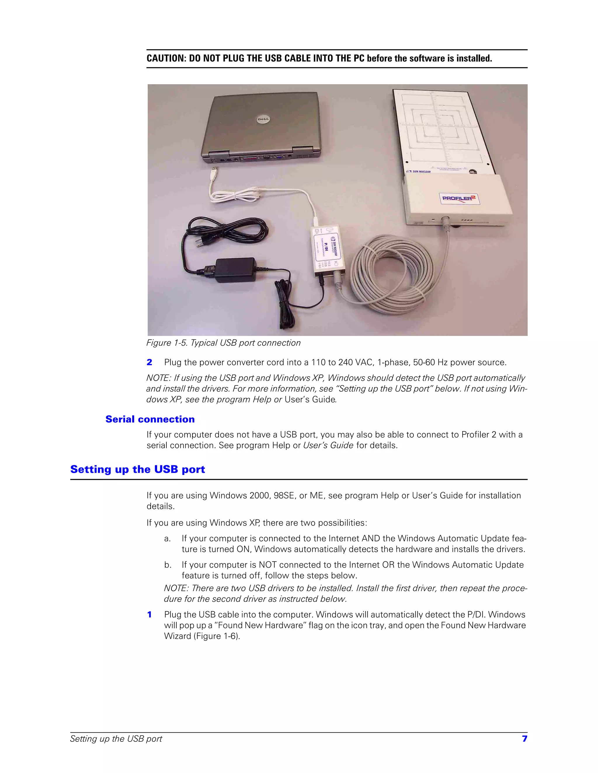
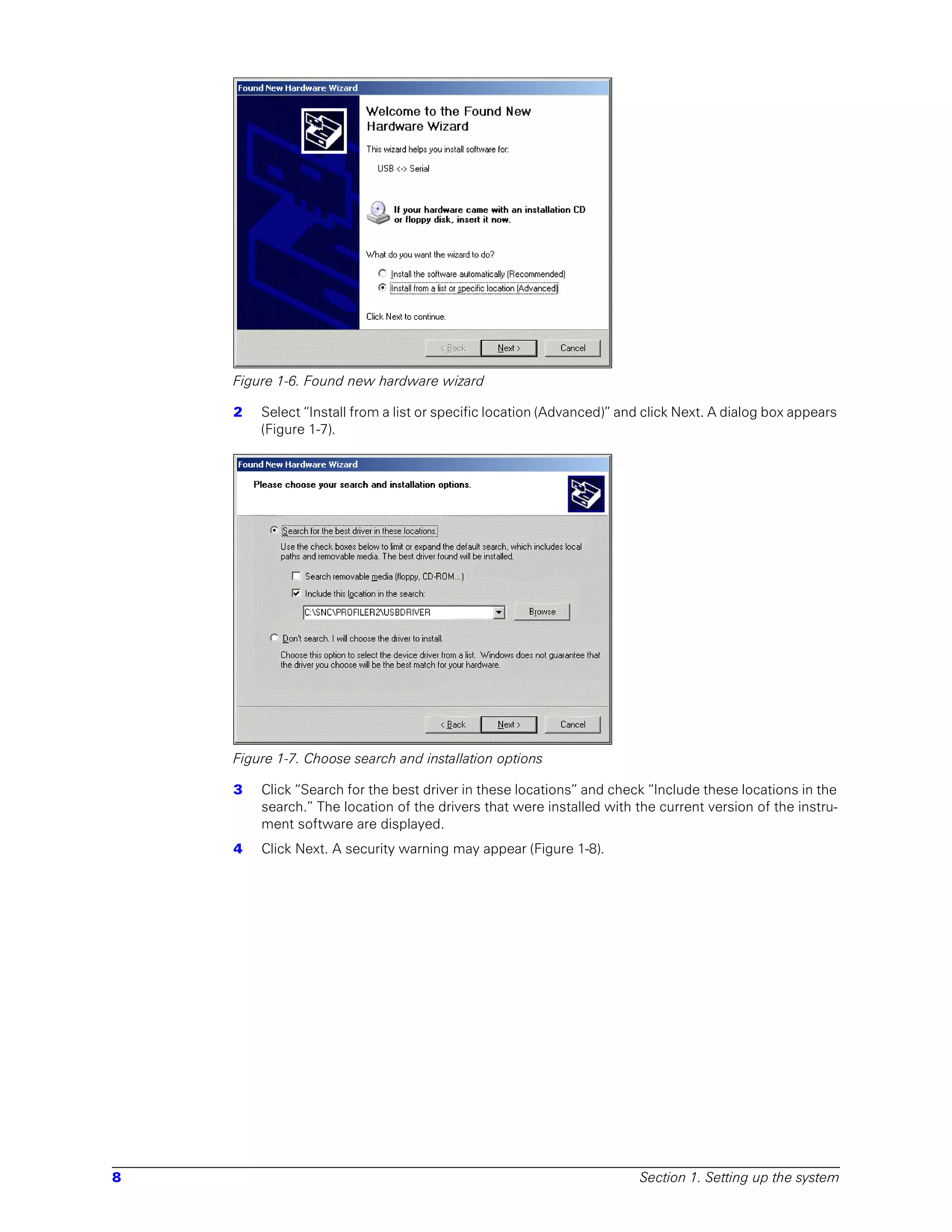
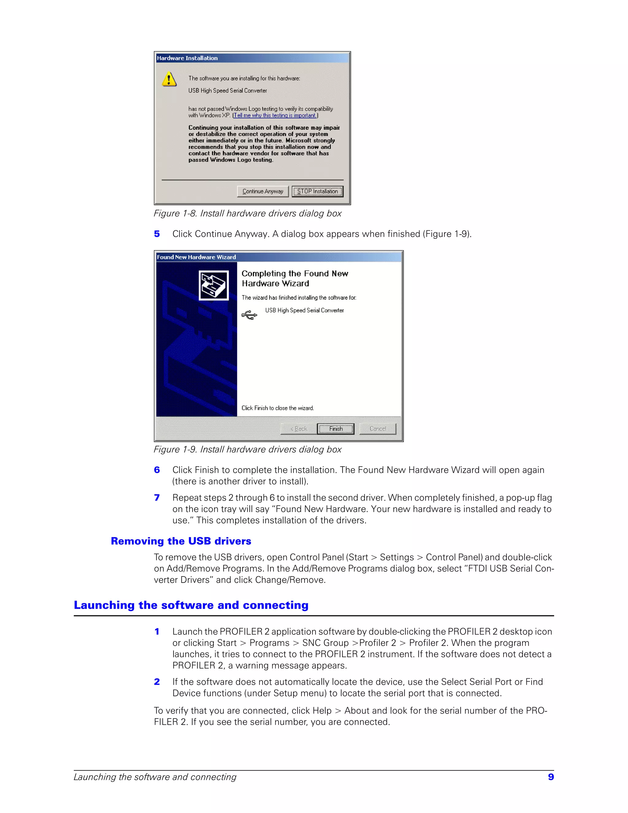
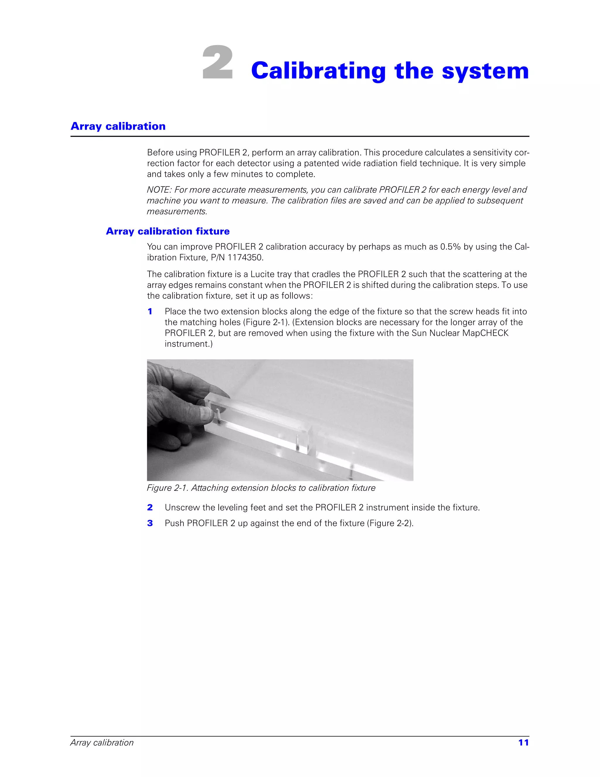
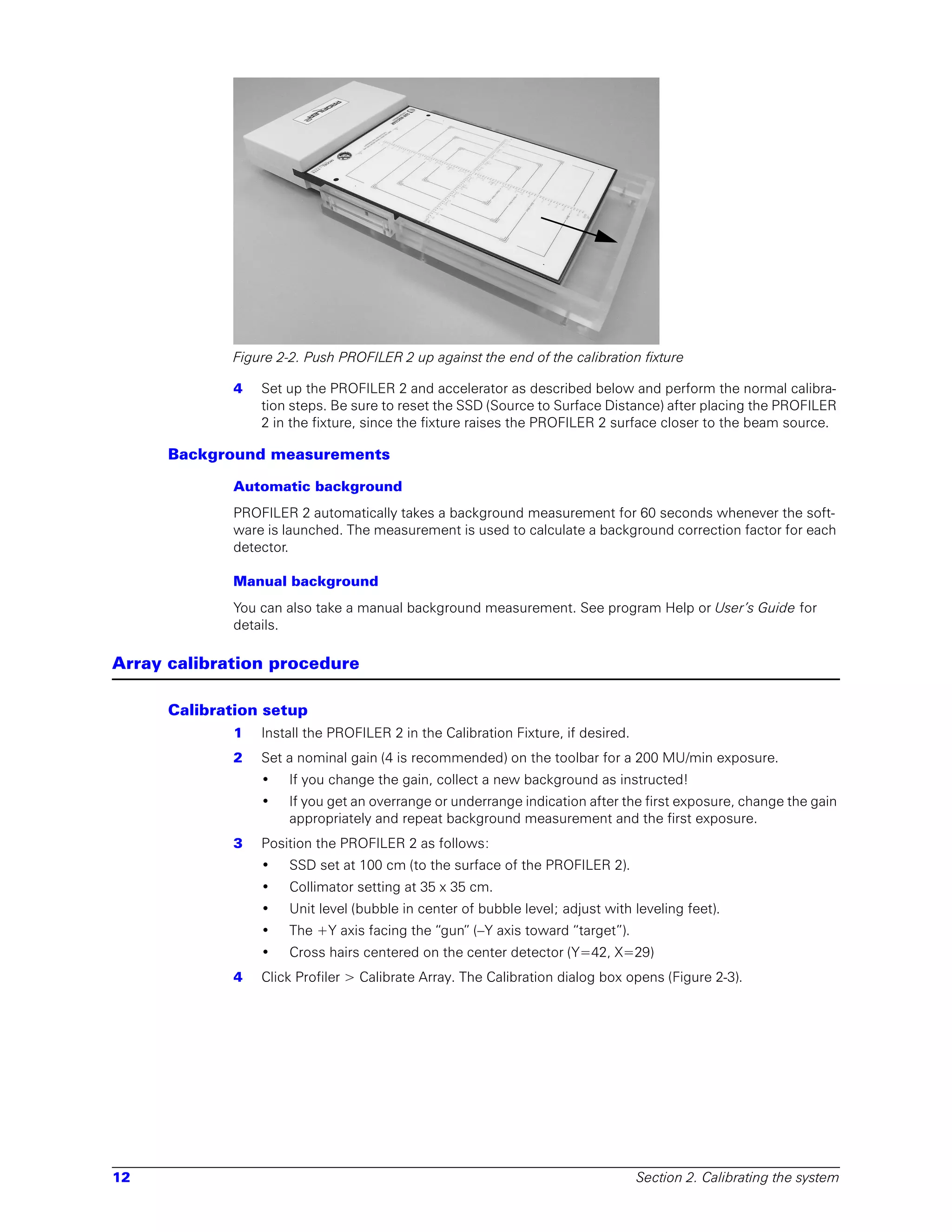

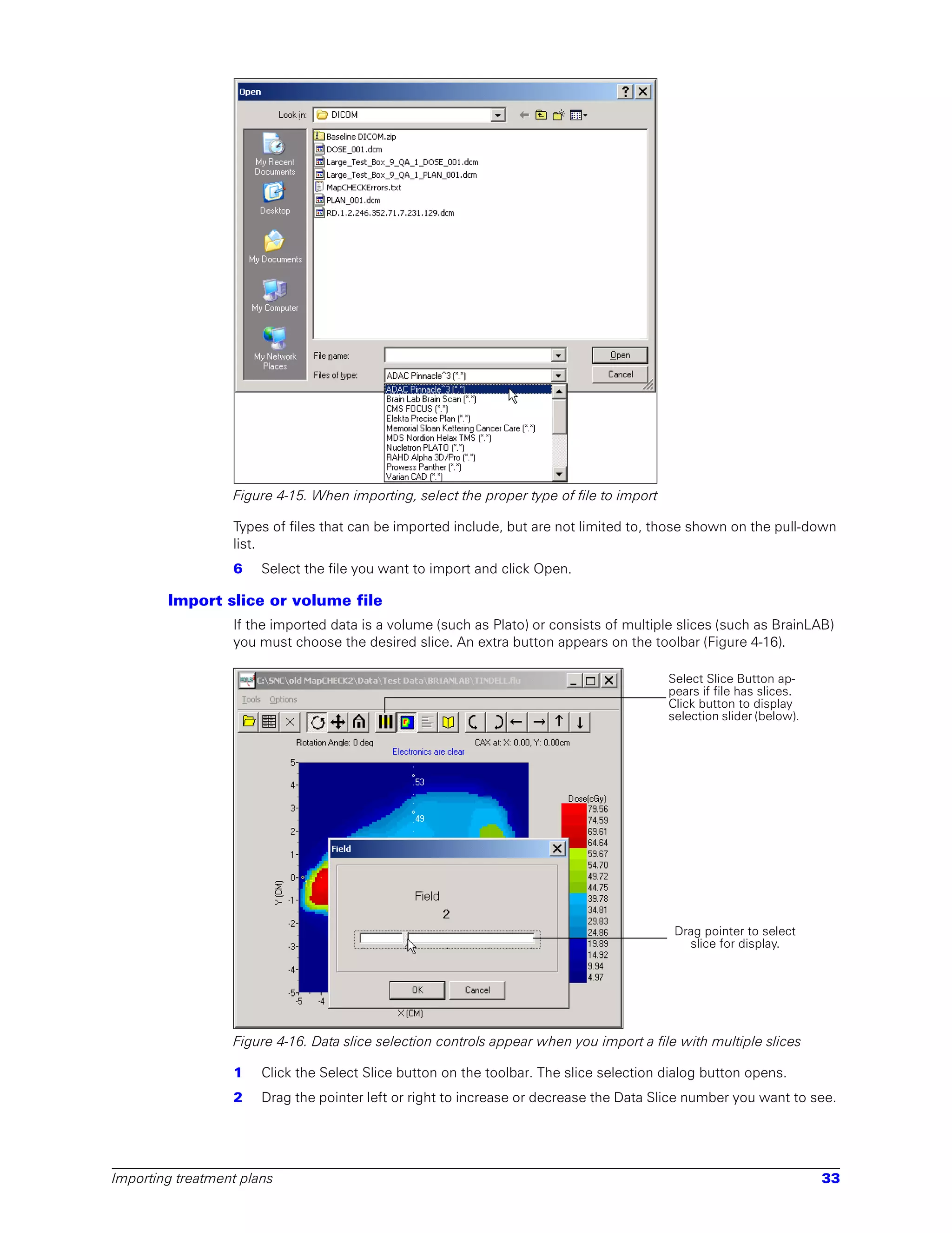
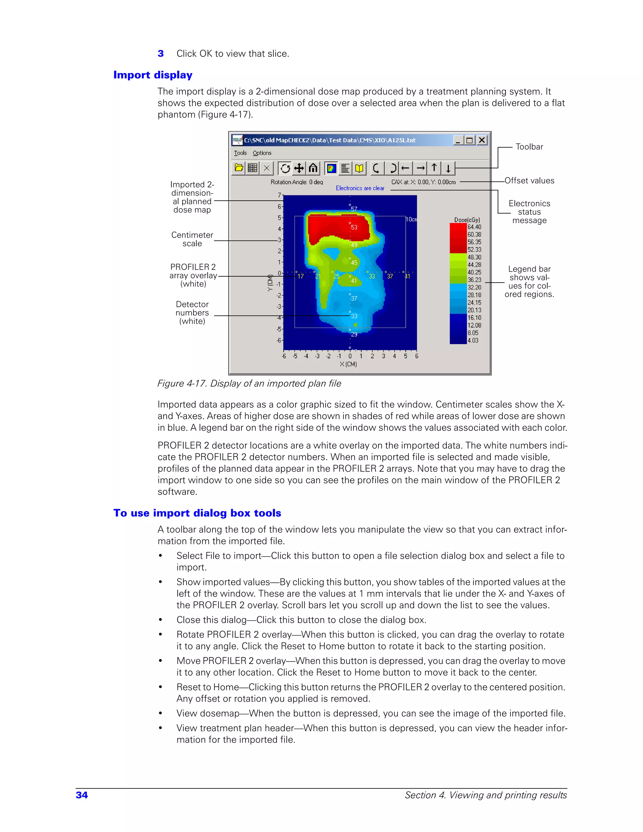
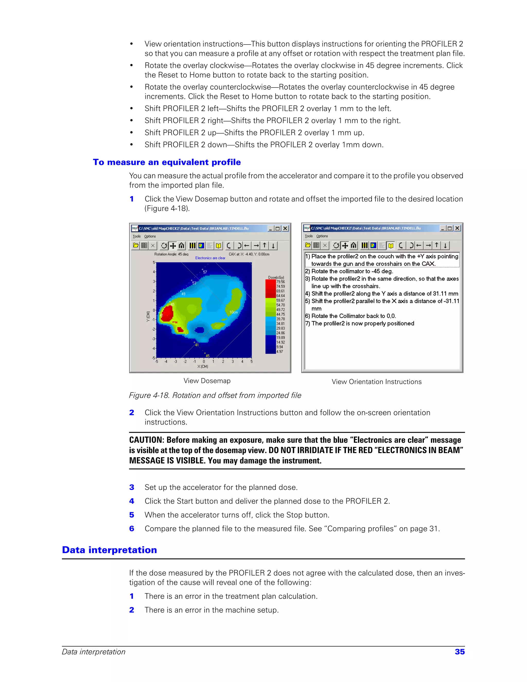


This document provides instructions for setting up the PROFILER 2 system, which includes a detector unit, cables, power/data interface, and software. It describes connecting the hardware components, installing the software, performing initial calibration of the detector array and dose calibration, and taking basic radiation measurements. The document also provides specifications for the PROFILER 2 detector array and operating instructions for the graphical user interface.


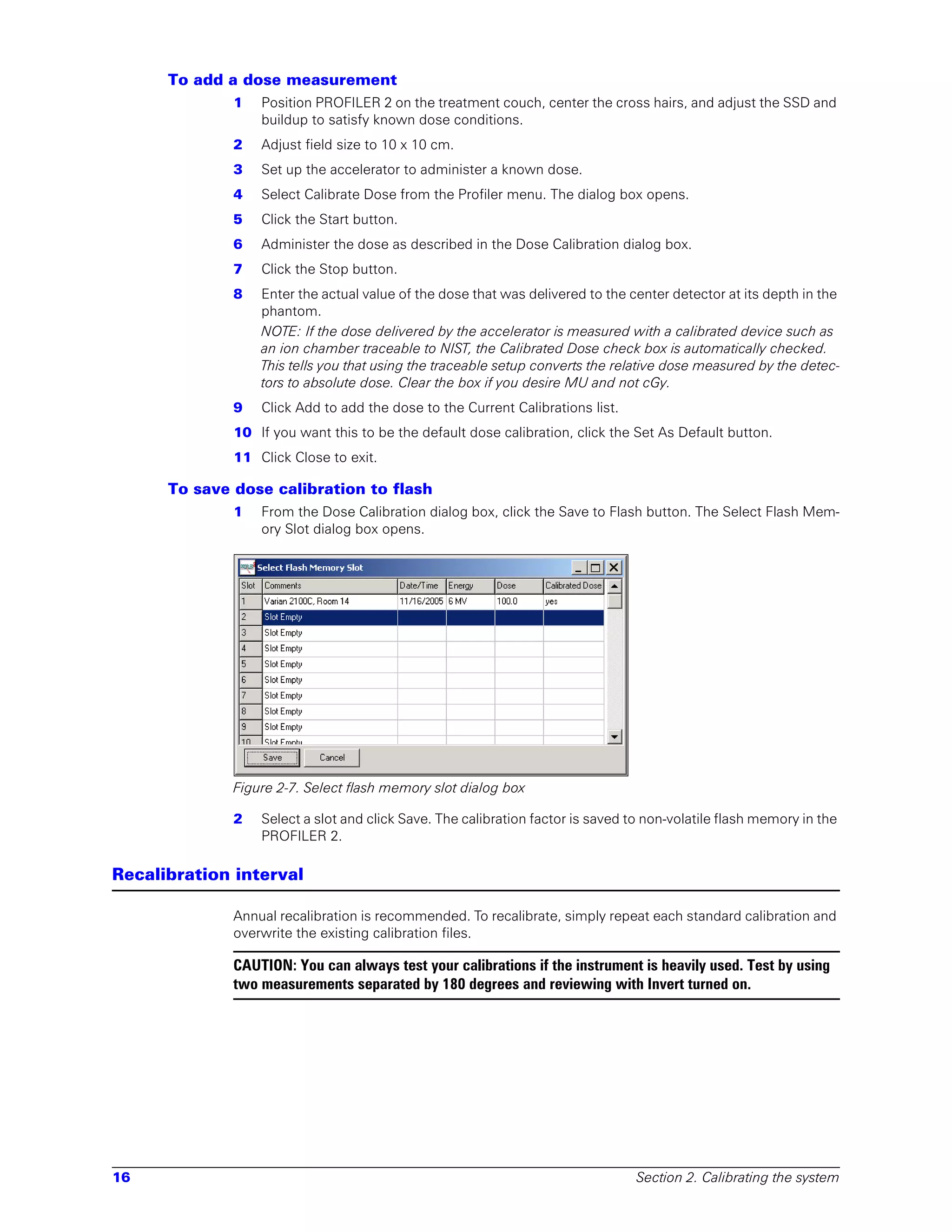
![Cimco edit 5 user guide[1]](https://cdn.slidesharecdn.com/ss_thumbnails/cimcoedit5userguide1-110305112440-phpapp01-thumbnail.jpg?width=640&height=640&fit=bounds)


