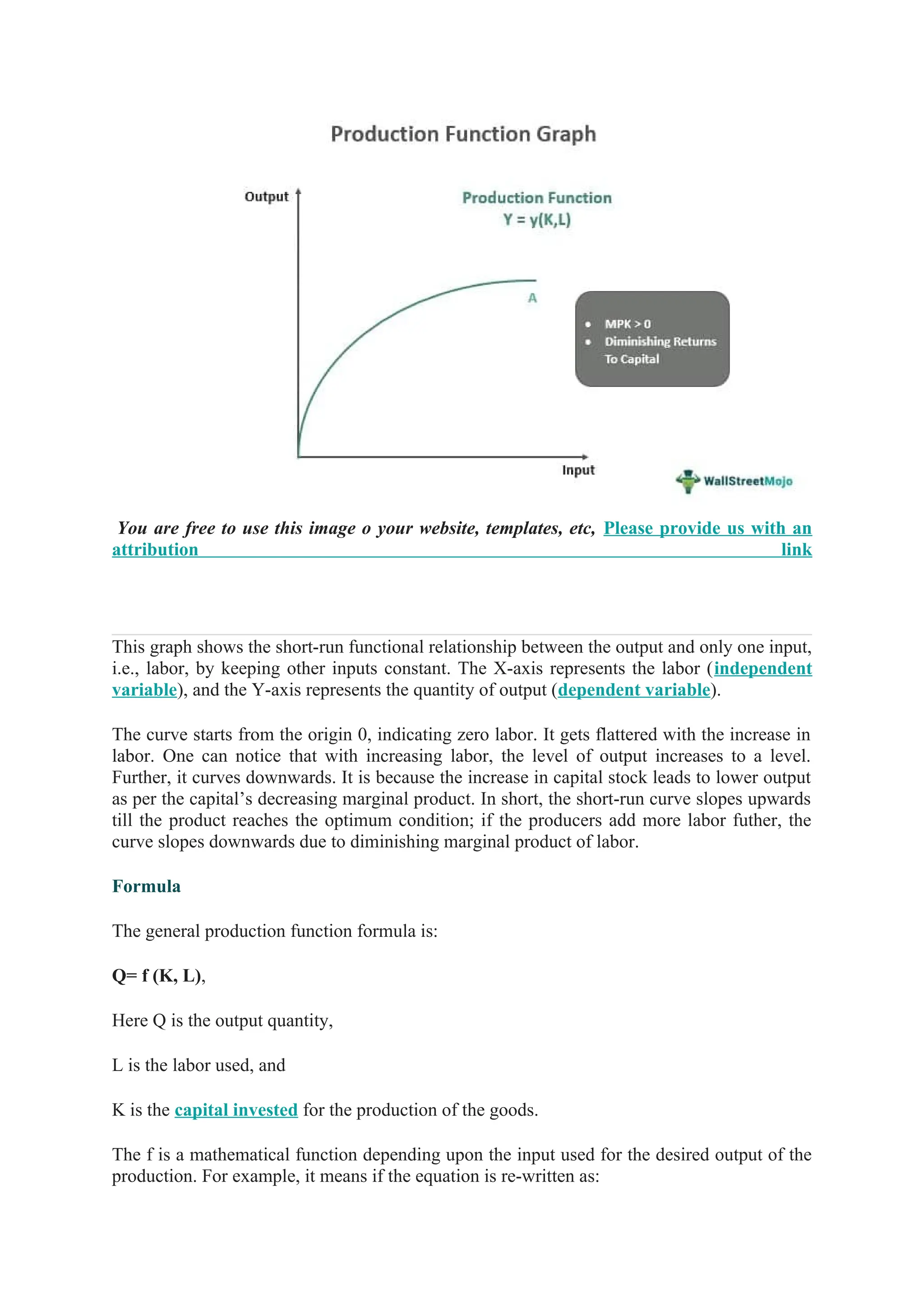
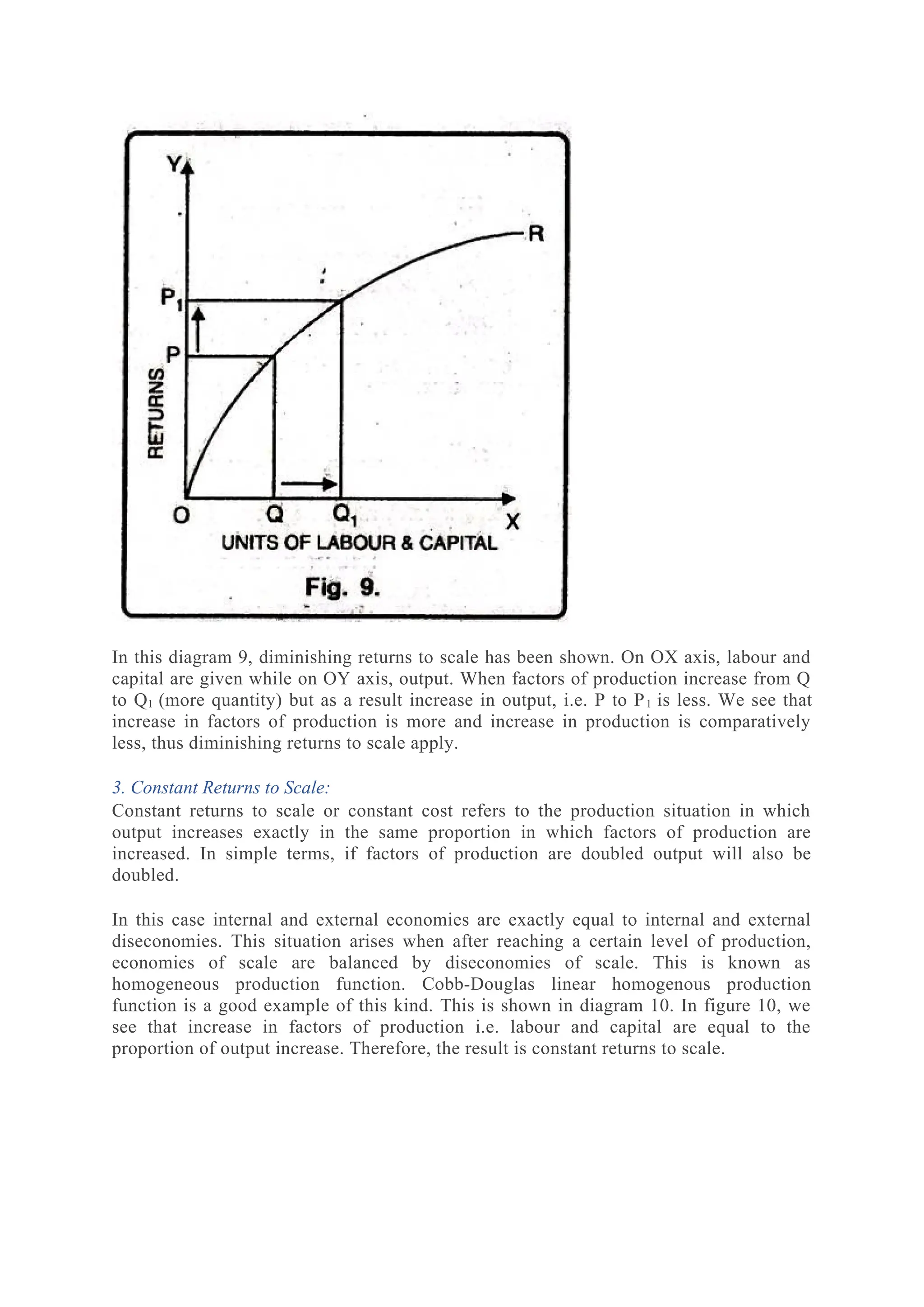
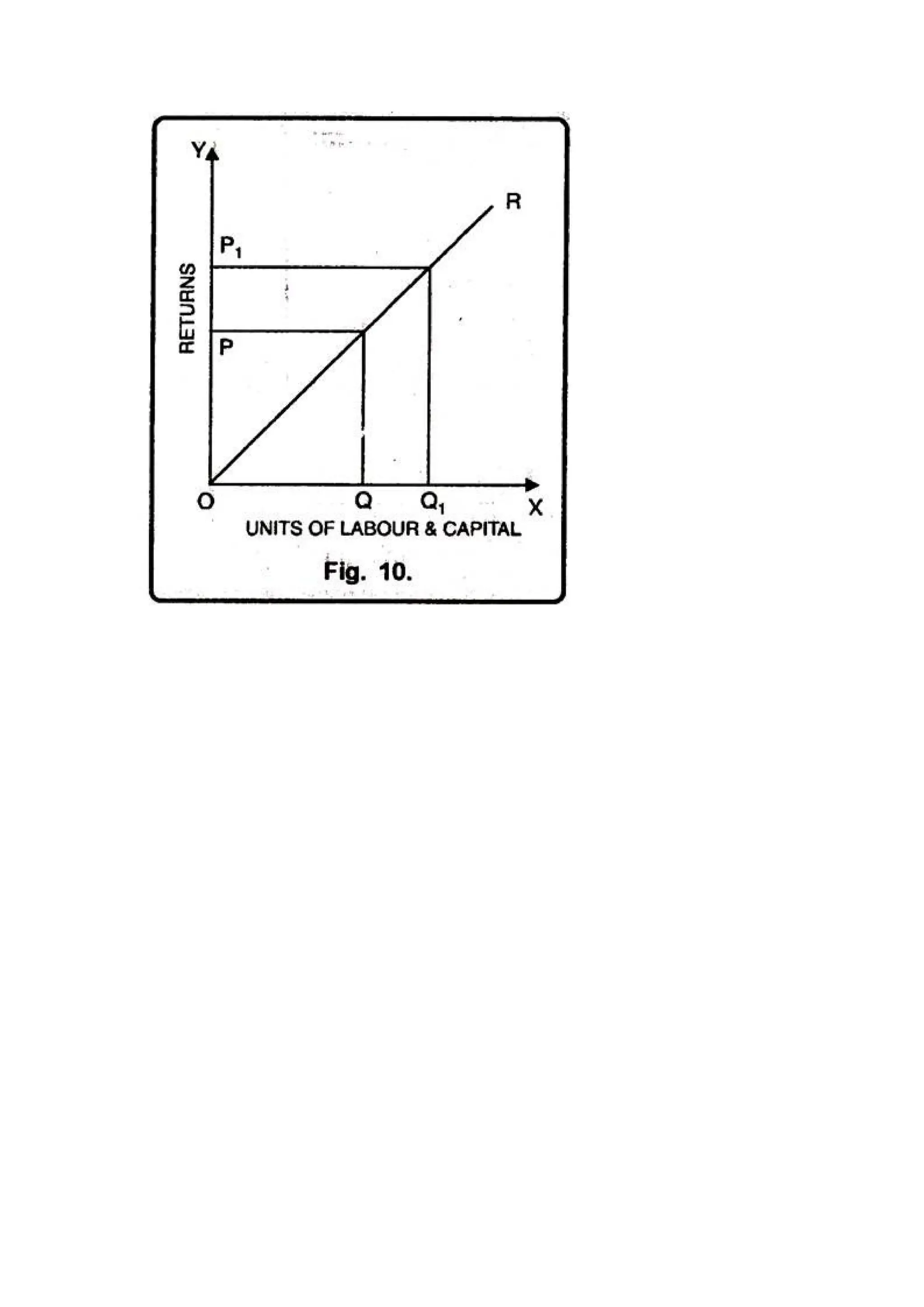
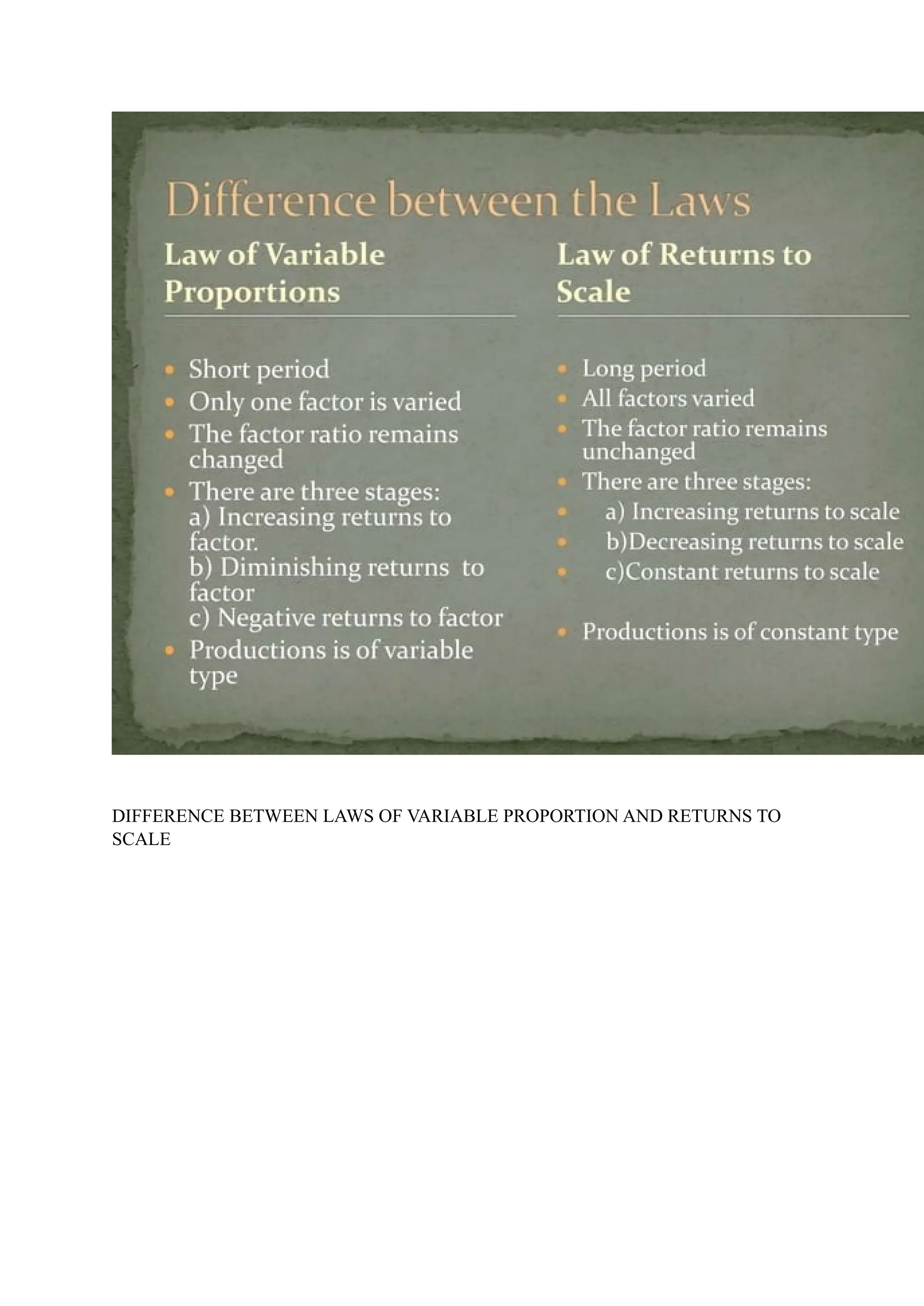
UNIT IV SYLLABUS
THEORY OF PRODUCTION
Concept of Production functions: Linear and Non-Linear homogeneous production
functions of a variable proportion of returns to scale -Difference between laws of
variable proportion and returns to scale -Economies of scale -Internal and external
economies-Internal and external diseconomies-Producer’s equilibrium
Introduction
Production is the process of converting inputs into outputs. The initial factors of production
results in final goods in the process of production. Production is a very important concept in
economics because it is the running force. Without production, economics cannot be
complete as economics starts with the production function and derives the other factors from
it.
Meaning of Production: What is the concept of production?
Any human initiative that creates a good for use can be called production. It requires four
factors as inputs, namely, land, labor, entrepreneurship, and capital to complete the initial
phase of production. The end product or goods are known as outputs in economics.
Production can result in output in the form of goods and services. Goods are products we can
view and touch with our hands such as mobiles, shirts, rice, utensils, etc. while we cannot see
services but can feel their use or presence. Teaching, medical services, transportation, etc.,
are forms of various services.
Three Types of Production Processes
Production processes can be classified into three types, which are the following:
Primary Production
Primary production processes tap or harness natural resources. It is related to obtaining
natural resources in the form of raw materials.
Examples of primary production include cultivation, mining, fishing, etc.
Secondary Production
This type of production converts primary resources, such as raw materials into finished
goods.
Examples include the production of railroads, houses, automobiles, shirts, and furniture. In
this type of production, the raw material goes through extraction and manufacturing.
Tertiary Production
This type of production concept is related to the services.
Examples of tertiary production include servicemen like teachers, doctors, soldiers, police,
hairdressers, etc.
The production concept refers to the production of goods at a mass scale so that the producers
can create demand for their products in the markets. This concept was pretty applicable in the
twentieth century.
However, in the twenty-first century, most companies have robust production and distribution
channels and therefore companies cannot beat their competitors depending on the concept of
production alone.
Examples of the Concept of Production
 A solid example of the concept of production is the outsourcing of services from one
company to another for the reason that the outsourcing company can save enough by
letting the other company do the task more efficiently.
For example, Apple produces most of its phones in Asia but sells them all over the
world. Here, manufacturing is outsourced to China and it is a glaring example of the
concept of production.
 Another similar example is the outsourcing of ITES projects of renowned US
companies to India. By harnessing the knowledge and power of Indian employees at a
fraction of the cost, US-based companies are earning huge profits. It is also an
example of the concept of production.
 If we look back to history, there are many examples of the concept of production. One
such example was related to the Ford Motor Company. The Ford Motor Company
started producing cars at economies of scale at the beginning of the twentieth century
believing that the more it produces, the more people will buy the cars.
This idea was true. At the beginning of the twentieth century, there was so much
demand for cars and so little availability that Ford Motor Company became one of the
most successful automobile companies in history. Believing in the concept of
production brought high dividends to Ford Motor Car Company.
PRODUCTION FUNCTION
Production function means a mathematical equation/representation of the relationship
between tangible inputs and the tangible output of a firm during the production of goods. A
single factor in the absence of the other three cannot help production. In simple words, it
describes the method that will enable the maximum production of goods by technically
combining the four major factors of production- land, enterprise, labor and capital at a
certain timeframe using a specific technology most efficiently. It changes with development
in technology. J H Von was the first person to develop the proportions of the first variable of
this function in the 1840s.
This function depends on the price factor and output levels that producers can easily observe.
Moreover, every manufacturing plant converts inputs into outputs. Hence the factors
necessarily determine the production level of goods to maximize profits and minimize cost.
Therefore, the production function is essential to know the quantity of output the firms
require to produce at the said price of goods. It determines the output and the combination
inputs at a certain capital and labor cost.
It is a common phenomenon that a firm’s marginal cost starts to increase at higher
production levels, which is known as diminishing returns to scale. The diminishing returns to
scale lead to a lesser proportional increase in output quantity by increasing the input
quantities. Moreover, the increase in marginal cost is identifiable by using this function.
Playvolume00:00/00:00wallstreetmojoTruvidfullScreen
The Leontief production function is a type of function that determines the ratio of input
required for producing in a unit of the output quantity. Also, producers and analysts use the
Cobb-Douglas function to calculate the aggregate production function.
Production Function Graph
Here is the production function graph to explain this concept of production:
You are free to use this image o your website, templates, etc, Please provide us with an
attribution link
This graph shows the short-run functional relationship between the output and only one input,
i.e., labor, by keeping other inputs constant. The X-axis represents the labor (independent
variable), and the Y-axis represents the quantity of output (dependent variable).
The curve starts from the origin 0, indicating zero labor. It gets flattered with the increase in
labor. One can notice that with increasing labor, the level of output increases to a level.
Further, it curves downwards. It is because the increase in capital stock leads to lower output
as per the capital’s decreasing marginal product. In short, the short-run curve slopes upwards
till the product reaches the optimum condition; if the producers add more labor futher, the
curve slopes downwards due to diminishing marginal product of labor.
Formula
The general production function formula is:
Q= f (K, L),
Here Q is the output quantity,
L is the labor used, and
K is the capital invested for the production of the goods.
The f is a mathematical function depending upon the input used for the desired output of the
production. For example, it means if the equation is re-written as:
Q= K+ L for a firm if the company uses two units of investment, K, and five units of labor.
As a result, the producer can produce 5+2 = 7 units of goods. Hence, increasing production
factors – labor and capital- will increase the quantity produced.
Another formula that this function uses is the Cobb-Douglas function denoted by:
Y= AK α L β,
Where A is the technology improvement factor,
K is the capital,
L is the labor,
Alpha (α) is the capital-output elasticity, and Beta (β) is the labor elasticity output.
One must always note that α + β is:
One under constant returns to scale
>1 under decreasing returns to scale and
<1 under increasing returns to scale
Example
Here is a production function example to understand the concept better.
Let us consider a famous garments company that produces the latest designer wear for
American customers. It requires three types of inputs for producing the designer garments:
cloth, industrial sewing machine, and tailor as an employee.
The variables- cloth, tailor, and industrial sewing machine is the variable that combines to
constitute the function. The Production function will then determine the quantity of output of
garments as per the number of inputs used. The industrial sewing machine can sew ten pieces
of garments every hour. The tailor can use these sewing machines to produce upto five pieces
of garment every 15 minutes. The length of clothing that the tailor will use per piece of
garment will be 2 meters. After including the data into the above formula, which is
Quantity of output, Q = min (input-1, input-2, input-3) where input1= cloth, input 2=
industrial sewing machine and input 3 = tailor
Production function Q, in one hour = min (input 1, input 2, input 3) = min (cloth+ tailor +
industrial sewing machine) = min (2mtrs per piece, 20 pieces by tailor, 20 pieces by machine)
= min (40 meters, 20 pieces, 20 pieces)
From the above, it is clear that if there are:
 Only 100 mtrs cloth are there then only 50 pieces of the garment can be made in 1
hour
 With only one machine, 20 pieces of production will take place in 1 hour.
 Only one tailor can help in the production of 20 pieces.
Therefore, the best product combination of the above three inputs – cloth, tailor, and
industrial sewing machine- is required to maximize the output of garments.
Types Of Production Function
There are two main types of productivity functions based on the input variables, as discussed
below.
#1 – Long Run
In the long-run production function, all the inputs are variable such as labor or raw
materials during a certain period. Therefore, the operation is flexible as all the input
variables can be changed per the firm’s requirements. Furthermore, in the production
function in economics, the producers can use the law of equi-marginal returns to scale. It
leads to a smaller rise in output if the producer increases the input even after the optimal
production capacity. It means the manufacturer can secure the best combination of factors
and change the production scale at any time. Therefore, the factor ratio remains the same
here.
Moreover, the firms are free to enter and exit in the long run due to low barriers.
#2 – Short Run
The firm cannot vary its input quantities in the short-run production function. The law of
variable proportion gets applicable here. There is no change in the level of activity in the
short-run function. The ratio of factors keeps changing because only one input changes
concerning all the other variables, which remain fixed. The manufacturing firms face exit
barriers. As a result, they can be shut down permanently but cannot exit from production.
For any production company, only the nature of the input variable determines the type of
productivity function one uses. If one uses variable input, it is a short-run productivity
function; otherwise, it is a long-run function
Overview of linear and non – linear functions
When plotted on a graph, a linear function is a function that produces a straight line.
Non-linear functions, on the other hand, are any functions that are not linear.
TABLE OF CONTENT
 What is a nonlinear function?
 Linear function table
 Non linear function equation
Something that is linear is something that is related to a line. For the purpose of constructing a
line, all of the linear equations are used. A nonlinear equation is one that does not have a
straight line as its solution. It has the appearance of a graph curve and has a variable slope
value, just like a graph.
In most cases, a linear equation contains only one variable, and if an equation contains two
variables, the equation is referred to as a Linear equation with two variables (or a Linear
equation with two variables). For example, the linear equation 5x + 2 = 1 is a one-variable linear
equation. 5x + 2y = 1, on the other hand, is a Linear equation in two variables.
What is a nonlinear function?
A nonlinear function is defined as a function whose graph does not consist of a single straight
line. Its graph does not have to be a straight line; it can be any curve. Consider the case of a
pond with 100 fishes at the start of the season, which doubles in size every week. This situation
can be represented by the function f(x) = 100 (2)x, where x is the number of weeks in the season
and f(x) is the number of fishes. Let’s create a table and graph this function using the table as a
reference point.
X Y
0 100
1 200
2 400
3 800
So the graph of the table is,
The graph above does not represent a line, and as a result, it represents a nonlinear function.
Based on the graph above, we can conclude that the slope of a nonlinear function is not
uniformly distributed. A nonlinear function can be represented in a variety of ways, including a
table of values, an equation, and a graph.
Linear function table:
The following are the steps to take in order to determine if a table of values determines a linear
function:
 The differences among each two consecutive x values are to be determined.
 Calculate the differences between each pair of consecutive y-coordinates.
 Figure out what the corresponding ratios of the differences of y and the differences of x
are.
 If none of the ratios are the same, then the function is only linear in one direction.
Non linear function equation:
A linear function has the form f(x) = ax + b. A linear function has the form f(x) = ax + b. Because
a nonlinear function is a function that is not a linear function, the equation for a nonlinear function
can be anything that is NOT of the form f(x) = ax+b. The following are some examples of
nonlinear functions:
 Because it is a quadratic function, f(x) = x2 is a nonlinear function.
 Because it is an exponential function, f(x) = 2x is not a linear function.
 Because it is a cubic function, f(x) = x3 – 3x is nonlinear.
Linear and nonlinear function
difference:
Linear function Nonlinear function
A linear function is a function for which the graph is
represented by a straight line.
A nonlinear function is a function for whom the graph
does not contain a straight line as its graph.
In mathematical terms, it has the equation f(x) = ax + b. Its equation can take on any form, with the exception of
the form f(x) = ax + b, which is required.
The slope of the curve is constant between any two
points on the curve.
Every point on the graph has a different slope than the
other point on the graph.
It is necessary to note that the ratio of difference of y
and difference of x in a linear function table is a
constant.
The ratio of the difference of y and the difference of x in
the table of a nonlinear function is NOT a constant in thi
case.
Tips and tricks on nonlinear function:
 Nonlinearity is defined as the absence of a line in the graph of a function.
 Nonlinearity is defined as the absence of the equation of a function of the form f(x) = ax +
b in the equation of a function.
 The objective function z = ax + by may be either a linear function or a nonlinear function,
depending on the situation.
 Nonlinear functions include rational functions, polynomial functions, exponential
functions, logarithmic functions, and other types of functions that are not linear.
Conclusion:
When plotted on a graph, a linear function is a function that produces a straight line. Non-linear
functions, on the other hand, are any functions that are not linear. A nonlinear equation is one
that does not have a straight line as its solution. In most cases, a linear equation contains only
one variable, and if an equation contains two variables, the equation is referred to as a Linear
equation with two variables. A nonlinear function is defined as a function whose graph does not
consist of a single straight line. Its graph does not have to be a straight line; it can be any curve.
For determining a linear function, The differences among each two consecutive x values are to
be determined, Calculate the differences between each pair of consecutive y-coordinates, If none
of the ratios are the same, then the function is only linear in one direction.
Nonlinearity is defined as the absence of a line in the graph of a function. Nonlinearity is defined
as the absence of the equation of a function of the form f(x) = ax + b in the equation of a function.
The objective function z = ax + by may be either a linear function or a nonlinear function,
depending on the situation.
LAW OF VARIABLE PROPORTION
Law of Variable Proportion
Law of Variable Proportion is regarded as an important theory in Economics. It is referred to
as the law which states that when the quantity of one factor of production is increased, while
keeping all other factors constant, it will result in the decline of the marginal product of that
factor.
Law of variable proportion is also known as the Law of Proportionality. When the variable
factor becomes more, it can lead to negative value of the marginal product.
The law of variable proportion can be understood in the following way.
When variable factor is increased while keeping all other factors constant, the total product
will increase initially at an increasing rate, next it will be increasing at a diminishing rate and
eventually there will be decline in the rate of production.
Assumptions of Law of Variable Proportion
Law of variable proportion holds good under certain circumstances, which will be discussed
in the following lines.
1. Constant state of Technology: It is assumed that the state of technology will be constant and
with improvements in the technology, the production will improve.
2. Variable Factor Proportions: This assumes that factors of production are variable. The law is
not valid, if factors of production are fixed.
3. Homogeneous factor units: This assumes that all the units produced are identical in quality,
quantity and price. In other words, the units are homogeneous in nature.
4. Short Run: This assumes that this law is applicable for those systems that are operating for a
short term, where it is not possible to alter all factor inputs.
Stages of Law of Variable Proportion
The Law of Variable proportions has three stages, which are discussed below.
1. First Stage or Stage of Increasing returns: In this stage, the total product increases at an
increasing rate. This happens because the efficiency of the fixed factors increases with
addition of variable inputs to the product.
2. Second Stage or Stage of Diminishing Returns: In this stage, the total product increases at a
diminishing rate until it reaches the maximum point. The marginal and average product are
positive but diminishing gradually.
3. Third Stage or Stage of Negative Returns: In this stage, the total product declines and the
marginal product becomes negative.
This concludes the topic of Law of Variable Proportions, which is an important concept for
the students of Commerce.
Explanation of the Law:
In order to understand the law of variable proportions we take the example of
agriculture. Suppose land and labour are the only two factors of production.
By keeping land as a fixed factor, the production of variable factor i.e., labour can
be shown with the help of the following table:
From the table 1 it is clear that there are three stages of the law of variable proportion. In
the first stage average production increases as there are more and more doses of labour
and capital employed with fixed factors (land). We see that total product, average
product, and marginal product increases but average product and marginal product
increases up to 40 units. Later on, both start decreasing because proportion of workers to
land was sufficient and land is not properly used. This is the end of the first stage.
The second stage starts from where the first stage ends or where AP=MP. In this stage,
average product and marginal product start falling. We should note that marginal product
falls at a faster rate than the average product. Here, total product increases at a
diminishing rate. It is also maximum at 70 units of labour where marginal product
becomes zero while average product is never zero or negative.
The third stage begins where second stage ends. This starts from 8th unit. Here, marginal
product is negative and total product falls but average product is still positive. At this
stage, any additional dose leads to positive nuisance because additional dose leads to
negative marginal product.
Graphic Presentation:
In fig. 1, on OX axis, we have measured number of labourers while quantity of product
is shown on OY axis. TP is total product curve. Up to point ‘E’, total product is
increasing at increasing rate. Between points E and G it is increasing at the decreasing
rate. Here marginal product has started falling. At point ‘G’ i.e., when 7 units of
labourers are employed, total product is maximum while, marginal product is zero.
Thereafter, it begins to diminish corresponding to negative marginal product. In the
lower part of the figure MP is marginal product curve.
Up to point ‘H’ marginal product increases. At point ‘H’, i.e., when 3 units of labourers
are employed, it is maximum. After that, marginal product begins to decrease. Before
point ‘I’ marginal product becomes zero at point C and it turns negative. AP curve
represents average product. Before point ‘I’, average product is less than marginal
product. At point ‘I’ average product is maximum. Up to point T, average product
increases but after that it starts to diminish.
LAWS OF RETURNS TO SCALE
Returns to scale refer to the change in output that results from a change in the factor inputs
simultaneously in the same proportion in the long run. Simply put, when a firm changes the
quantity of all inputs in the long run, it changes the scale of production for the goods.
The law of variable proportions emerges because factor proportions change as long as one
factor is held unchanged and the other is raised. What if both factors can change (differ)?
Always remember that this can occur only in the long run. One special case, in the long run,
happens when both the factors are raised by the same amount of factors are ascended up.
When a proportionate increase in all inputs results in the rise in output by the same
proportion, the production function is said to exhibit Constant returns to scale (CRS).
When a proportionate increase in all inputs results in the rise in output by the larger
proportion, the production function is said to exhibit an Increasing Returns to Scale (IRS).
Decreasing Returns to Scale (DRS) occurs when a proportionate increase in all inputs results
in a rise in output by a smaller proportion.
For instance, presume in a manufacturing procedure, all inputs get doubled. As an outcome, if
the output gets doubled, the manufacturing procedure displays CRS. If the output is less than
doubled, then DRS occurs and if it is more than doubled, then IRS occurs.
LAWS OF RETURNS TO SCALE
The term returns to scale refers to the changes in output as all factors change by the same
proportion.” Koutsoyiannis
“Returns to scale relates to the behaviour of total output as all inputs are varied and is a
long run concept”. Leibhafsky
ADVERTISEMENTS:
Returns to scale are of the following three types:
1. Increasing Returns to scale.
2. Constant Returns to Scale
3. Diminishing Returns to Scale
Explanation:
In the long run, output can be increased by increasing all factors in the same proportion.
Generally, laws of returns to scale refer to an increase in output due to increase in all
factors in the same proportion. Such an increase is called returns to scale.
ADVERTISEMENTS:
Suppose, initially production function is as follows:
P = f (L, K)
Now, if both the factors of production i.e., labour and capital are increased in same
proportion i.e., x, product function will be rewritten as.
The above stated table explains the following three stages of returns to scale:
1. Increasing Returns to Scale:
Increasing returns to scale or diminishing cost refers to a situation when all factors of
production are increased, output increases at a higher rate. It means if all inputs are
doubled, output will also increase at the faster rate than double. Hence, it is said to be
increasing returns to scale. This increase is due to many reasons like division external
economies of scale. Increasing returns to scale can be illustrated with the help of a
diagram 8.
In figure 8, OX axis represents increase in labour and capital while OY axis shows
increase in output. When labour and capital increases from Q to Q1, output also increases
from P to P1 which is higher than the factors of production i.e. labour and capital.
2. Diminishing Returns to Scale:
Diminishing returns or increasing costs refer to that production situation, where if all the
factors of production are increased in a given proportion, output increases in a smaller
proportion. It means, if inputs are doubled, output will be less than doubled. If 20
percent increase in labour and capital is followed by 10 percent increase in output, then it
is an instance of diminishing returns to scale.
The main cause of the operation of diminishing returns to scale is that internal and
external economies are less than internal and external diseconomies. It is clear from
diagram 9.
In this diagram 9, diminishing returns to scale has been shown. On OX axis, labour and
capital are given while on OY axis, output. When factors of production increase from Q
to Q1 (more quantity) but as a result increase in output, i.e. P to P1 is less. We see that
increase in factors of production is more and increase in production is comparatively
less, thus diminishing returns to scale apply.
3. Constant Returns to Scale:
Constant returns to scale or constant cost refers to the production situation in which
output increases exactly in the same proportion in which factors of production are
increased. In simple terms, if factors of production are doubled output will also be
doubled.
In this case internal and external economies are exactly equal to internal and external
diseconomies. This situation arises when after reaching a certain level of production,
economies of scale are balanced by diseconomies of scale. This is known as
homogeneous production function. Cobb-Douglas linear homogenous production
function is a good example of this kind. This is shown in diagram 10. In figure 10, we
see that increase in factors of production i.e. labour and capital are equal to the
proportion of output increase. Therefore, the result is constant returns to scale.
DIFFERENCE BETWEEN LAWS OF VARIABLE PROPORTION AND RETURNS TO
SCALE
ECONOMIES OF SCALE
Economies of scale may be defined as the cost advantages that can be achieved by an
organisation by the expansion of their production in the long run. Therefore, the advantages
of large scale expansion are known as Economies of Scale. The lower average cost per unit
achieves the advantage in cost.
Economies of Scale are a long term concept that is achieved when there is an increase in the
sales of an organisation. Due to the lowering of production cost, the organisation can save
more and invest it in buying a bulk of raw materials which can again be obtained at a
discount.
These are the benefits of Economies of Scale. When there is a massive expansion in an
organisation, the cost per unit may increase with the increase in output. Diseconomies of
Scale may arise due to internal issues resulting from technical, organisational, or resource
constraints.
Types of Economies of Scale
The Economies of Scale may be divided into two categories-
1) Internal Economies
2) External Economies.
Internal Economies: Internal Economies are the real economies that arise from the
expansion of the organisation. These economies are the result of the growth of the
organisation itself.
External Economics: External Economics are the economies that originate from factors
outside the organisation. These economies result in the increase in the main organisation by
the increase in the quality of factors outside the organisation like better transportation, better
labour, infrastructure, etc. Due to the betterment of these external factors, the cost of
production per unit of an item in the organisation decreases.
DISECONOMIES OF SCALE
Diseconomies of scale happen when a company or business grows so large that the costs per
unit increase. It takes place when economies of scale no longer function for a firm. With this
principle, rather than experiencing continued decreasing costs and increasing output, a firm
sees an increase in costs when output is increased.
Types of Diseconomies of Scale
Similar to the Economies of Scale, Diseconomies of Scale is of two types- Internal
Diseconomies of Scale and External Diseconomies of Scale.
Internal Diseconomies of Scale:
Internal Diseconomies of Scale are the Diseconomies resulting from the internal difficulties
within the organisation. The Internal Diseconomies are the factors that raise the cost of
production of an organisation like lack of supervision, lack of management and technical
difficulties.
External Diseconomies of Scale:
External Diseconomies of Scale are the external factors that result in the increase in the
production per unit of a product within an organisation. The external factors that act as a
restrain to expansion may include the cost of production per unit, scarcity of raw materials,
and low availability of skilled labours.
Solved Examples
Q1. What are the Factors which differ between Internal and External Economies of
Scale?
Answer: Economies of Scale are of two types, namely Internal and External Economies of
Scale. Internal Economies of Scale originate from internal factors within the organisation.
The Internal Economies of Scale are the internal factors that can be controlled by the
organisation to lower the cost of production.
On the other hand, External Economies of Scale are the external factors that affect the cost of
production per unit. The External Economies of Scale are the factors that reduce the cost of
production. Unlike internal Economies of Scale, the External Economies of scale cannot be
controlled by the organisation. They include factors like the availability of highly skilled
labour, tax reductions, partnerships, etc. any factor that can reduce the cost of production per
unit.
Examples of Internal Economies
Technical Economies of Scale: This occurs when an organisation invests in modern
technology which helps in lowering the cost of production. It enables an organisation to
produce a large number of goods in a lesser period.
Financial Economies of Scale: This occurs when large organisations take a loan with a low
rate of interest. The banks easily give them loans since they have good credibility.
Managerial Economies of Scale: This occurs when large organisations employ people with
a special skill set that helps to maximize the profits of the organisation like an accountant or
manager.
Marketing Economies of Scale: This occurs when large organisations increase their budget.
They can then spread their market by setting up branches or buying more raw materials in
bulk at a lower price.
Cournot Dilemma
It has also highlighted that in several industrial areas there exist several enterprises with
varying sizes and organizational structures. This conflict, among the actual data and the
conceptual opposition among economies of scale and competitiveness, has been termed the
‘Cournot dilemma’. Whereas the study is expanded, including the issues involving the
growth of information and the structuring of interactions, it is possible to infer that economies
of scale do not necessarily result in dominance. In reality, the comparative benefits resulting
from the growth of the firm's competencies and from the administration of dealings with
suppliers and consumers might offset those supplied by the scale. Thereby it neutralizes the
inclination to a monopoly implicit in economies of scale.
In other words, the variability of the organizational forms and of the size of the firms
functioning in a field of business can be decided by variables concerning the reliability of the
goods, the manufacturing flexibility, the contractual methods, the educational opportunities,
the heterogeneity of choices of clients who convey a distinguishable requirement with respect
to the reliability of the product, and aid before and after the sale. Such as, for instance,
flexible production on a large scale, small-scale adaptable production, mass production,
industrial production predicated on strict technologies affiliated with flexible organizational
systems and related artisan production.
Solutions to Diseconomies of Scale
Approaches to the diseconomies of scale for large organizations may entail separating the
corporation into smaller groups. This can either occur by consequence when the firm is in
financial problems, sells off its successful sections, or closes down the remainder. It can also
happen intentionally if the management is willing. To prevent the adverse consequences of
diseconomies of scale, a business must keep to the lowest average production cost. It must
strive to detect any external diseconomies of scale. Furthermore, on obtaining the lowest
average cost, a business must either extend to other nations to generate demand for its
products or explore new markets or manufacture new items that do not conflict with its
original products. Nevertheless, neither of these activities would definitely eradicate
connectivity and management challenges commonly associated with huge firms.
A comprehensive examination and redesign of business operations, in order to minimize
complication, can offset diseconomies of scale. This allows for greater productivity. Better
management systems and more effective supervision of labour and activities can decrease
costs.
BUSINESS ECONOMICS NOTES UNIT IV (1)DB JAIN COLLEGE.DOCX

BUSINESS ECONOMICS NOTES UNIT IV (1)DB JAIN COLLEGE.DOCX

  • 1.
    UNIT IV SYLLABUS THEORYOF PRODUCTION Concept of Production functions: Linear and Non-Linear homogeneous production functions of a variable proportion of returns to scale -Difference between laws of variable proportion and returns to scale -Economies of scale -Internal and external economies-Internal and external diseconomies-Producer’s equilibrium Introduction Production is the process of converting inputs into outputs. The initial factors of production results in final goods in the process of production. Production is a very important concept in economics because it is the running force. Without production, economics cannot be complete as economics starts with the production function and derives the other factors from it. Meaning of Production: What is the concept of production? Any human initiative that creates a good for use can be called production. It requires four factors as inputs, namely, land, labor, entrepreneurship, and capital to complete the initial phase of production. The end product or goods are known as outputs in economics. Production can result in output in the form of goods and services. Goods are products we can view and touch with our hands such as mobiles, shirts, rice, utensils, etc. while we cannot see services but can feel their use or presence. Teaching, medical services, transportation, etc., are forms of various services. Three Types of Production Processes Production processes can be classified into three types, which are the following: Primary Production Primary production processes tap or harness natural resources. It is related to obtaining natural resources in the form of raw materials. Examples of primary production include cultivation, mining, fishing, etc. Secondary Production
  • 2.
    This type ofproduction converts primary resources, such as raw materials into finished goods. Examples include the production of railroads, houses, automobiles, shirts, and furniture. In this type of production, the raw material goes through extraction and manufacturing. Tertiary Production This type of production concept is related to the services. Examples of tertiary production include servicemen like teachers, doctors, soldiers, police, hairdressers, etc. The production concept refers to the production of goods at a mass scale so that the producers can create demand for their products in the markets. This concept was pretty applicable in the twentieth century. However, in the twenty-first century, most companies have robust production and distribution channels and therefore companies cannot beat their competitors depending on the concept of production alone. Examples of the Concept of Production  A solid example of the concept of production is the outsourcing of services from one company to another for the reason that the outsourcing company can save enough by letting the other company do the task more efficiently. For example, Apple produces most of its phones in Asia but sells them all over the world. Here, manufacturing is outsourced to China and it is a glaring example of the concept of production.  Another similar example is the outsourcing of ITES projects of renowned US companies to India. By harnessing the knowledge and power of Indian employees at a fraction of the cost, US-based companies are earning huge profits. It is also an example of the concept of production.  If we look back to history, there are many examples of the concept of production. One such example was related to the Ford Motor Company. The Ford Motor Company started producing cars at economies of scale at the beginning of the twentieth century believing that the more it produces, the more people will buy the cars. This idea was true. At the beginning of the twentieth century, there was so much demand for cars and so little availability that Ford Motor Company became one of the most successful automobile companies in history. Believing in the concept of production brought high dividends to Ford Motor Car Company.
  • 3.
    PRODUCTION FUNCTION Production functionmeans a mathematical equation/representation of the relationship between tangible inputs and the tangible output of a firm during the production of goods. A
  • 4.
    single factor inthe absence of the other three cannot help production. In simple words, it describes the method that will enable the maximum production of goods by technically combining the four major factors of production- land, enterprise, labor and capital at a certain timeframe using a specific technology most efficiently. It changes with development in technology. J H Von was the first person to develop the proportions of the first variable of this function in the 1840s. This function depends on the price factor and output levels that producers can easily observe. Moreover, every manufacturing plant converts inputs into outputs. Hence the factors necessarily determine the production level of goods to maximize profits and minimize cost. Therefore, the production function is essential to know the quantity of output the firms require to produce at the said price of goods. It determines the output and the combination inputs at a certain capital and labor cost. It is a common phenomenon that a firm’s marginal cost starts to increase at higher production levels, which is known as diminishing returns to scale. The diminishing returns to scale lead to a lesser proportional increase in output quantity by increasing the input quantities. Moreover, the increase in marginal cost is identifiable by using this function. Playvolume00:00/00:00wallstreetmojoTruvidfullScreen The Leontief production function is a type of function that determines the ratio of input required for producing in a unit of the output quantity. Also, producers and analysts use the Cobb-Douglas function to calculate the aggregate production function. Production Function Graph Here is the production function graph to explain this concept of production:
  • 5.
    You are freeto use this image o your website, templates, etc, Please provide us with an attribution link This graph shows the short-run functional relationship between the output and only one input, i.e., labor, by keeping other inputs constant. The X-axis represents the labor (independent variable), and the Y-axis represents the quantity of output (dependent variable). The curve starts from the origin 0, indicating zero labor. It gets flattered with the increase in labor. One can notice that with increasing labor, the level of output increases to a level. Further, it curves downwards. It is because the increase in capital stock leads to lower output as per the capital’s decreasing marginal product. In short, the short-run curve slopes upwards till the product reaches the optimum condition; if the producers add more labor futher, the curve slopes downwards due to diminishing marginal product of labor. Formula The general production function formula is: Q= f (K, L), Here Q is the output quantity, L is the labor used, and K is the capital invested for the production of the goods. The f is a mathematical function depending upon the input used for the desired output of the production. For example, it means if the equation is re-written as:
  • 6.
    Q= K+ Lfor a firm if the company uses two units of investment, K, and five units of labor. As a result, the producer can produce 5+2 = 7 units of goods. Hence, increasing production factors – labor and capital- will increase the quantity produced. Another formula that this function uses is the Cobb-Douglas function denoted by: Y= AK α L β, Where A is the technology improvement factor, K is the capital, L is the labor, Alpha (α) is the capital-output elasticity, and Beta (β) is the labor elasticity output. One must always note that α + β is: One under constant returns to scale >1 under decreasing returns to scale and <1 under increasing returns to scale Example Here is a production function example to understand the concept better. Let us consider a famous garments company that produces the latest designer wear for American customers. It requires three types of inputs for producing the designer garments: cloth, industrial sewing machine, and tailor as an employee. The variables- cloth, tailor, and industrial sewing machine is the variable that combines to constitute the function. The Production function will then determine the quantity of output of garments as per the number of inputs used. The industrial sewing machine can sew ten pieces of garments every hour. The tailor can use these sewing machines to produce upto five pieces of garment every 15 minutes. The length of clothing that the tailor will use per piece of garment will be 2 meters. After including the data into the above formula, which is Quantity of output, Q = min (input-1, input-2, input-3) where input1= cloth, input 2= industrial sewing machine and input 3 = tailor Production function Q, in one hour = min (input 1, input 2, input 3) = min (cloth+ tailor + industrial sewing machine) = min (2mtrs per piece, 20 pieces by tailor, 20 pieces by machine) = min (40 meters, 20 pieces, 20 pieces) From the above, it is clear that if there are:
  • 7.
     Only 100mtrs cloth are there then only 50 pieces of the garment can be made in 1 hour  With only one machine, 20 pieces of production will take place in 1 hour.  Only one tailor can help in the production of 20 pieces. Therefore, the best product combination of the above three inputs – cloth, tailor, and industrial sewing machine- is required to maximize the output of garments. Types Of Production Function There are two main types of productivity functions based on the input variables, as discussed below. #1 – Long Run In the long-run production function, all the inputs are variable such as labor or raw materials during a certain period. Therefore, the operation is flexible as all the input variables can be changed per the firm’s requirements. Furthermore, in the production function in economics, the producers can use the law of equi-marginal returns to scale. It leads to a smaller rise in output if the producer increases the input even after the optimal production capacity. It means the manufacturer can secure the best combination of factors and change the production scale at any time. Therefore, the factor ratio remains the same here. Moreover, the firms are free to enter and exit in the long run due to low barriers. #2 – Short Run The firm cannot vary its input quantities in the short-run production function. The law of variable proportion gets applicable here. There is no change in the level of activity in the short-run function. The ratio of factors keeps changing because only one input changes concerning all the other variables, which remain fixed. The manufacturing firms face exit barriers. As a result, they can be shut down permanently but cannot exit from production. For any production company, only the nature of the input variable determines the type of productivity function one uses. If one uses variable input, it is a short-run productivity function; otherwise, it is a long-run function
  • 8.
    Overview of linearand non – linear functions When plotted on a graph, a linear function is a function that produces a straight line. Non-linear functions, on the other hand, are any functions that are not linear. TABLE OF CONTENT  What is a nonlinear function?  Linear function table  Non linear function equation Something that is linear is something that is related to a line. For the purpose of constructing a line, all of the linear equations are used. A nonlinear equation is one that does not have a straight line as its solution. It has the appearance of a graph curve and has a variable slope value, just like a graph. In most cases, a linear equation contains only one variable, and if an equation contains two variables, the equation is referred to as a Linear equation with two variables (or a Linear equation with two variables). For example, the linear equation 5x + 2 = 1 is a one-variable linear equation. 5x + 2y = 1, on the other hand, is a Linear equation in two variables. What is a nonlinear function? A nonlinear function is defined as a function whose graph does not consist of a single straight line. Its graph does not have to be a straight line; it can be any curve. Consider the case of a pond with 100 fishes at the start of the season, which doubles in size every week. This situation can be represented by the function f(x) = 100 (2)x, where x is the number of weeks in the season and f(x) is the number of fishes. Let’s create a table and graph this function using the table as a reference point. X Y 0 100 1 200 2 400 3 800 So the graph of the table is,
  • 9.
    The graph abovedoes not represent a line, and as a result, it represents a nonlinear function. Based on the graph above, we can conclude that the slope of a nonlinear function is not uniformly distributed. A nonlinear function can be represented in a variety of ways, including a table of values, an equation, and a graph. Linear function table: The following are the steps to take in order to determine if a table of values determines a linear function:  The differences among each two consecutive x values are to be determined.  Calculate the differences between each pair of consecutive y-coordinates.  Figure out what the corresponding ratios of the differences of y and the differences of x are.  If none of the ratios are the same, then the function is only linear in one direction. Non linear function equation: A linear function has the form f(x) = ax + b. A linear function has the form f(x) = ax + b. Because a nonlinear function is a function that is not a linear function, the equation for a nonlinear function can be anything that is NOT of the form f(x) = ax+b. The following are some examples of nonlinear functions:  Because it is a quadratic function, f(x) = x2 is a nonlinear function.  Because it is an exponential function, f(x) = 2x is not a linear function.  Because it is a cubic function, f(x) = x3 – 3x is nonlinear. Linear and nonlinear function difference: Linear function Nonlinear function A linear function is a function for which the graph is represented by a straight line. A nonlinear function is a function for whom the graph does not contain a straight line as its graph.
  • 10.
    In mathematical terms,it has the equation f(x) = ax + b. Its equation can take on any form, with the exception of the form f(x) = ax + b, which is required. The slope of the curve is constant between any two points on the curve. Every point on the graph has a different slope than the other point on the graph. It is necessary to note that the ratio of difference of y and difference of x in a linear function table is a constant. The ratio of the difference of y and the difference of x in the table of a nonlinear function is NOT a constant in thi case. Tips and tricks on nonlinear function:  Nonlinearity is defined as the absence of a line in the graph of a function.  Nonlinearity is defined as the absence of the equation of a function of the form f(x) = ax + b in the equation of a function.  The objective function z = ax + by may be either a linear function or a nonlinear function, depending on the situation.  Nonlinear functions include rational functions, polynomial functions, exponential functions, logarithmic functions, and other types of functions that are not linear. Conclusion: When plotted on a graph, a linear function is a function that produces a straight line. Non-linear functions, on the other hand, are any functions that are not linear. A nonlinear equation is one that does not have a straight line as its solution. In most cases, a linear equation contains only one variable, and if an equation contains two variables, the equation is referred to as a Linear equation with two variables. A nonlinear function is defined as a function whose graph does not consist of a single straight line. Its graph does not have to be a straight line; it can be any curve. For determining a linear function, The differences among each two consecutive x values are to be determined, Calculate the differences between each pair of consecutive y-coordinates, If none of the ratios are the same, then the function is only linear in one direction. Nonlinearity is defined as the absence of a line in the graph of a function. Nonlinearity is defined as the absence of the equation of a function of the form f(x) = ax + b in the equation of a function. The objective function z = ax + by may be either a linear function or a nonlinear function, depending on the situation.
  • 11.
    LAW OF VARIABLEPROPORTION Law of Variable Proportion Law of Variable Proportion is regarded as an important theory in Economics. It is referred to as the law which states that when the quantity of one factor of production is increased, while keeping all other factors constant, it will result in the decline of the marginal product of that factor. Law of variable proportion is also known as the Law of Proportionality. When the variable factor becomes more, it can lead to negative value of the marginal product. The law of variable proportion can be understood in the following way. When variable factor is increased while keeping all other factors constant, the total product will increase initially at an increasing rate, next it will be increasing at a diminishing rate and eventually there will be decline in the rate of production. Assumptions of Law of Variable Proportion Law of variable proportion holds good under certain circumstances, which will be discussed in the following lines. 1. Constant state of Technology: It is assumed that the state of technology will be constant and with improvements in the technology, the production will improve. 2. Variable Factor Proportions: This assumes that factors of production are variable. The law is not valid, if factors of production are fixed. 3. Homogeneous factor units: This assumes that all the units produced are identical in quality, quantity and price. In other words, the units are homogeneous in nature. 4. Short Run: This assumes that this law is applicable for those systems that are operating for a short term, where it is not possible to alter all factor inputs. Stages of Law of Variable Proportion The Law of Variable proportions has three stages, which are discussed below. 1. First Stage or Stage of Increasing returns: In this stage, the total product increases at an increasing rate. This happens because the efficiency of the fixed factors increases with addition of variable inputs to the product. 2. Second Stage or Stage of Diminishing Returns: In this stage, the total product increases at a diminishing rate until it reaches the maximum point. The marginal and average product are positive but diminishing gradually.
  • 12.
    3. Third Stageor Stage of Negative Returns: In this stage, the total product declines and the marginal product becomes negative. This concludes the topic of Law of Variable Proportions, which is an important concept for the students of Commerce. Explanation of the Law: In order to understand the law of variable proportions we take the example of agriculture. Suppose land and labour are the only two factors of production. By keeping land as a fixed factor, the production of variable factor i.e., labour can be shown with the help of the following table: From the table 1 it is clear that there are three stages of the law of variable proportion. In the first stage average production increases as there are more and more doses of labour and capital employed with fixed factors (land). We see that total product, average product, and marginal product increases but average product and marginal product increases up to 40 units. Later on, both start decreasing because proportion of workers to land was sufficient and land is not properly used. This is the end of the first stage. The second stage starts from where the first stage ends or where AP=MP. In this stage, average product and marginal product start falling. We should note that marginal product falls at a faster rate than the average product. Here, total product increases at a diminishing rate. It is also maximum at 70 units of labour where marginal product becomes zero while average product is never zero or negative. The third stage begins where second stage ends. This starts from 8th unit. Here, marginal product is negative and total product falls but average product is still positive. At this stage, any additional dose leads to positive nuisance because additional dose leads to negative marginal product.
  • 13.
    Graphic Presentation: In fig.1, on OX axis, we have measured number of labourers while quantity of product is shown on OY axis. TP is total product curve. Up to point ‘E’, total product is increasing at increasing rate. Between points E and G it is increasing at the decreasing rate. Here marginal product has started falling. At point ‘G’ i.e., when 7 units of labourers are employed, total product is maximum while, marginal product is zero. Thereafter, it begins to diminish corresponding to negative marginal product. In the lower part of the figure MP is marginal product curve. Up to point ‘H’ marginal product increases. At point ‘H’, i.e., when 3 units of labourers are employed, it is maximum. After that, marginal product begins to decrease. Before point ‘I’ marginal product becomes zero at point C and it turns negative. AP curve represents average product. Before point ‘I’, average product is less than marginal product. At point ‘I’ average product is maximum. Up to point T, average product increases but after that it starts to diminish.
  • 14.
    LAWS OF RETURNSTO SCALE Returns to scale refer to the change in output that results from a change in the factor inputs simultaneously in the same proportion in the long run. Simply put, when a firm changes the quantity of all inputs in the long run, it changes the scale of production for the goods. The law of variable proportions emerges because factor proportions change as long as one factor is held unchanged and the other is raised. What if both factors can change (differ)? Always remember that this can occur only in the long run. One special case, in the long run, happens when both the factors are raised by the same amount of factors are ascended up. When a proportionate increase in all inputs results in the rise in output by the same proportion, the production function is said to exhibit Constant returns to scale (CRS). When a proportionate increase in all inputs results in the rise in output by the larger proportion, the production function is said to exhibit an Increasing Returns to Scale (IRS). Decreasing Returns to Scale (DRS) occurs when a proportionate increase in all inputs results in a rise in output by a smaller proportion. For instance, presume in a manufacturing procedure, all inputs get doubled. As an outcome, if the output gets doubled, the manufacturing procedure displays CRS. If the output is less than doubled, then DRS occurs and if it is more than doubled, then IRS occurs. LAWS OF RETURNS TO SCALE The term returns to scale refers to the changes in output as all factors change by the same proportion.” Koutsoyiannis “Returns to scale relates to the behaviour of total output as all inputs are varied and is a long run concept”. Leibhafsky ADVERTISEMENTS: Returns to scale are of the following three types: 1. Increasing Returns to scale. 2. Constant Returns to Scale 3. Diminishing Returns to Scale
  • 15.
    Explanation: In the longrun, output can be increased by increasing all factors in the same proportion. Generally, laws of returns to scale refer to an increase in output due to increase in all factors in the same proportion. Such an increase is called returns to scale. ADVERTISEMENTS: Suppose, initially production function is as follows: P = f (L, K) Now, if both the factors of production i.e., labour and capital are increased in same proportion i.e., x, product function will be rewritten as. The above stated table explains the following three stages of returns to scale: 1. Increasing Returns to Scale: Increasing returns to scale or diminishing cost refers to a situation when all factors of production are increased, output increases at a higher rate. It means if all inputs are doubled, output will also increase at the faster rate than double. Hence, it is said to be increasing returns to scale. This increase is due to many reasons like division external economies of scale. Increasing returns to scale can be illustrated with the help of a diagram 8.
  • 16.
    In figure 8,OX axis represents increase in labour and capital while OY axis shows increase in output. When labour and capital increases from Q to Q1, output also increases from P to P1 which is higher than the factors of production i.e. labour and capital. 2. Diminishing Returns to Scale: Diminishing returns or increasing costs refer to that production situation, where if all the factors of production are increased in a given proportion, output increases in a smaller proportion. It means, if inputs are doubled, output will be less than doubled. If 20 percent increase in labour and capital is followed by 10 percent increase in output, then it is an instance of diminishing returns to scale. The main cause of the operation of diminishing returns to scale is that internal and external economies are less than internal and external diseconomies. It is clear from diagram 9.
  • 17.
    In this diagram9, diminishing returns to scale has been shown. On OX axis, labour and capital are given while on OY axis, output. When factors of production increase from Q to Q1 (more quantity) but as a result increase in output, i.e. P to P1 is less. We see that increase in factors of production is more and increase in production is comparatively less, thus diminishing returns to scale apply. 3. Constant Returns to Scale: Constant returns to scale or constant cost refers to the production situation in which output increases exactly in the same proportion in which factors of production are increased. In simple terms, if factors of production are doubled output will also be doubled. In this case internal and external economies are exactly equal to internal and external diseconomies. This situation arises when after reaching a certain level of production, economies of scale are balanced by diseconomies of scale. This is known as homogeneous production function. Cobb-Douglas linear homogenous production function is a good example of this kind. This is shown in diagram 10. In figure 10, we see that increase in factors of production i.e. labour and capital are equal to the proportion of output increase. Therefore, the result is constant returns to scale.
  • 19.
    DIFFERENCE BETWEEN LAWSOF VARIABLE PROPORTION AND RETURNS TO SCALE
  • 20.
    ECONOMIES OF SCALE Economiesof scale may be defined as the cost advantages that can be achieved by an organisation by the expansion of their production in the long run. Therefore, the advantages of large scale expansion are known as Economies of Scale. The lower average cost per unit achieves the advantage in cost. Economies of Scale are a long term concept that is achieved when there is an increase in the sales of an organisation. Due to the lowering of production cost, the organisation can save more and invest it in buying a bulk of raw materials which can again be obtained at a discount. These are the benefits of Economies of Scale. When there is a massive expansion in an organisation, the cost per unit may increase with the increase in output. Diseconomies of Scale may arise due to internal issues resulting from technical, organisational, or resource constraints. Types of Economies of Scale The Economies of Scale may be divided into two categories- 1) Internal Economies 2) External Economies. Internal Economies: Internal Economies are the real economies that arise from the expansion of the organisation. These economies are the result of the growth of the organisation itself. External Economics: External Economics are the economies that originate from factors outside the organisation. These economies result in the increase in the main organisation by the increase in the quality of factors outside the organisation like better transportation, better labour, infrastructure, etc. Due to the betterment of these external factors, the cost of production per unit of an item in the organisation decreases. DISECONOMIES OF SCALE Diseconomies of scale happen when a company or business grows so large that the costs per unit increase. It takes place when economies of scale no longer function for a firm. With this principle, rather than experiencing continued decreasing costs and increasing output, a firm sees an increase in costs when output is increased. Types of Diseconomies of Scale Similar to the Economies of Scale, Diseconomies of Scale is of two types- Internal Diseconomies of Scale and External Diseconomies of Scale. Internal Diseconomies of Scale: Internal Diseconomies of Scale are the Diseconomies resulting from the internal difficulties within the organisation. The Internal Diseconomies are the factors that raise the cost of production of an organisation like lack of supervision, lack of management and technical difficulties. External Diseconomies of Scale: External Diseconomies of Scale are the external factors that result in the increase in the production per unit of a product within an organisation. The external factors that act as a restrain to expansion may include the cost of production per unit, scarcity of raw materials, and low availability of skilled labours. Solved Examples
  • 21.
    Q1. What arethe Factors which differ between Internal and External Economies of Scale? Answer: Economies of Scale are of two types, namely Internal and External Economies of Scale. Internal Economies of Scale originate from internal factors within the organisation. The Internal Economies of Scale are the internal factors that can be controlled by the organisation to lower the cost of production. On the other hand, External Economies of Scale are the external factors that affect the cost of production per unit. The External Economies of Scale are the factors that reduce the cost of production. Unlike internal Economies of Scale, the External Economies of scale cannot be controlled by the organisation. They include factors like the availability of highly skilled labour, tax reductions, partnerships, etc. any factor that can reduce the cost of production per unit. Examples of Internal Economies Technical Economies of Scale: This occurs when an organisation invests in modern technology which helps in lowering the cost of production. It enables an organisation to produce a large number of goods in a lesser period. Financial Economies of Scale: This occurs when large organisations take a loan with a low rate of interest. The banks easily give them loans since they have good credibility. Managerial Economies of Scale: This occurs when large organisations employ people with a special skill set that helps to maximize the profits of the organisation like an accountant or manager. Marketing Economies of Scale: This occurs when large organisations increase their budget. They can then spread their market by setting up branches or buying more raw materials in bulk at a lower price. Cournot Dilemma It has also highlighted that in several industrial areas there exist several enterprises with varying sizes and organizational structures. This conflict, among the actual data and the conceptual opposition among economies of scale and competitiveness, has been termed the ‘Cournot dilemma’. Whereas the study is expanded, including the issues involving the growth of information and the structuring of interactions, it is possible to infer that economies of scale do not necessarily result in dominance. In reality, the comparative benefits resulting from the growth of the firm's competencies and from the administration of dealings with suppliers and consumers might offset those supplied by the scale. Thereby it neutralizes the inclination to a monopoly implicit in economies of scale. In other words, the variability of the organizational forms and of the size of the firms functioning in a field of business can be decided by variables concerning the reliability of the goods, the manufacturing flexibility, the contractual methods, the educational opportunities, the heterogeneity of choices of clients who convey a distinguishable requirement with respect to the reliability of the product, and aid before and after the sale. Such as, for instance, flexible production on a large scale, small-scale adaptable production, mass production, industrial production predicated on strict technologies affiliated with flexible organizational systems and related artisan production. Solutions to Diseconomies of Scale Approaches to the diseconomies of scale for large organizations may entail separating the corporation into smaller groups. This can either occur by consequence when the firm is in financial problems, sells off its successful sections, or closes down the remainder. It can also
  • 22.
    happen intentionally ifthe management is willing. To prevent the adverse consequences of diseconomies of scale, a business must keep to the lowest average production cost. It must strive to detect any external diseconomies of scale. Furthermore, on obtaining the lowest average cost, a business must either extend to other nations to generate demand for its products or explore new markets or manufacture new items that do not conflict with its original products. Nevertheless, neither of these activities would definitely eradicate connectivity and management challenges commonly associated with huge firms. A comprehensive examination and redesign of business operations, in order to minimize complication, can offset diseconomies of scale. This allows for greater productivity. Better management systems and more effective supervision of labour and activities can decrease costs.