Managerial Economics&Financial Analysis
1| Mohammad Imran
Production Function
Introduction
The production function expresses a functional relationship between physical inputs and physical
outputs of a firm at any particular time period. The output is thus a function of inputs.
Mathematically production function can be written as Q= f (A, B, C, D)
Where “Q” stands for the quantity of output and A, B, C, D are various input factors such as land, labour,
capital and organization.
Here output is the function of inputs. Hence output becomes the dependent variable and inputs are the
independent variables. The above function does not state by how much the output of “Q” changes as a
consequence of change of variable inputs. In order to express the quantitative relationship between inputs and
output, Production function has been expressed in a precise mathematical equation i.e. Y= a+b(x) Which shows
that there is a constant relationship between applications of input (the only factor input ‘X’ in this case) and the
amount of output (y) produced.
Importance:
1. When inputs are specified in physical units, production function helps to estimate the level of
production.
2. It becomes is equates when different combinations of inputs yield the same level of output.
3. It indicates the manner in which the firm can substitute on input for another without altering the total
output.
4. When price is taken into consideration, the production function helps to select the least combination
of inputs for the desired output.
5. It considers two types’ input-output relationships namely ‘law of variable proportions’ and ‘law of
returns to scale’. Law of variable propositions explains the pattern of output in the short-run as the units of
variable inputs are increased to increase the output. On the other hand law of returns to scale explains the
pattern of output in the long run as all the units of inputs are increased.
6. The production function explains the maximum quantity of output, which can be produced, from any
chosen quantities of various inputs or the minimum quantities of various inputs that are required to produce a
given quantity of output. Production function can be fitted the particular firm or industry or for the economy as
whole. Production function will change with an improvement in technology.
Assumptions: Production function has the following assumptions.
1. The production function is related to a particular period of time.
2. There is no change in technology.
3. The producer is using the best techniques available.
4. The factors of production are divisible.
5. Production function can be fitted to a short run or to long run.
Managerial Economics&Financial Analysis
2| Mohammad Imran
Cobb-Douglas production function:
Production function of the linear homogenous type is invested by Junt wicksell and first tested by C. W.
Cobb and P. H. Dougles in 1928.
This famous statistical production function is known as Cobb-Douglas production function. Originally the
function is applied on the empirical study of the American manufacturing industry. Cabb – Douglas production
function takes the following mathematical form.
Y= (AKX L1-x)
Where Y=output
K=Capital
L=Labour
A, ∞=positive constant
Assumptions:
It has the following assumptions
1. The function assumes that output is the function of two factors viz. capital and labour.
2. It is a linear homogenous production function of the first degree
3. The function assumes that the logarithm of the total output of the economy is a linear function of the
logarithms of the labour force and capital stock.
4. There are constant returns to scale
5. All inputs are homogenous
6. There is perfect competition
7. There is no change in technology
ISOQUANTS
The term Isoquants is derived from the words ‘iso’ and ‘quant’ – ‘Iso’ means equal and ‘quent’ implies
quantity. Isoquant therefore, means equal quantity. A family of iso-product curves or isoquants or production
difference curves can represent a production function with two variable inputs, which are substitutable for one
another within limits. Iqoquants are the curves, which represent the different combinations of inputs producing
a particular quantity of output. Any combination on the isoquant represents the some level of output. For a
given output level firm’s production become, Q= f (L, K) Where ‘Q’, the units of output is a function of the
quantity of two inputs ‘L’ and ‘K’. Thus an isoquant shows all possible combinations of two inputs, which are
capable of producing equal or a given level of output. Since each combination yields same output, the producer
becomes indifferent towards these combinations.
Assumptions:
1. there are only two factors of production, viz. labour and capital.
2. The two factors can substitute each other up to certain limit
3. The shape of the isoquant depends upon the extent of substitutability of the two inputs.
4. The technology is given over a period. An isoquant may be explained with the help of an arithmetical
Managerial Economics&Financial Analysis
3| Mohammad Imran
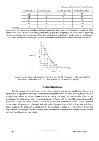
Example.
Combination ‘A’ represent 1 unit of labour and 10 units of capital and produces ‘50’ quintals of a product all other
combinations in the table are assumed to yield the same given output of a product say ‘50’ quintals by employing
any one of the alternative combinations of the two factors labour and capital. If we plot all these combinations
on a paper and join them, we will get continues and smooth curve called Iso-product curve as shown below.
Labour is on the X-axis and capital is on the Y-axis. IQ is the ISO-Product curve which shows all the
alternative combinations A, B, C, D, E which can produce 50 quintals of a product.
Producer’s Equilibrium:
The tem producer’s equilibrium is the counter part of consumer’s equilibrium. Just as the
consumer is in equilibrium when be secures maximum satisfaction, in the same manner, the producer is
in equilibrium when he secures maximum output, with the least cost combination of factors of
production. The optimum position of the producer can be found with the help of iso-product curve. The
Isoproduct curve or equal product curve or production indifference curve shows different
combinations of two factors of production, which yield the same output. This is illustrated as follows.
Let us suppose. The producer can produces the given output of paddy say 100 quintals by employing
any one of the following alternative combinations of the two factors labour and capital computation of
least cost combination of two inputs.

7 Production function

  • 1.
    Managerial Economics&Financial Analysis 1|Mohammad Imran Production Function Introduction The production function expresses a functional relationship between physical inputs and physical outputs of a firm at any particular time period. The output is thus a function of inputs. Mathematically production function can be written as Q= f (A, B, C, D) Where “Q” stands for the quantity of output and A, B, C, D are various input factors such as land, labour, capital and organization. Here output is the function of inputs. Hence output becomes the dependent variable and inputs are the independent variables. The above function does not state by how much the output of “Q” changes as a consequence of change of variable inputs. In order to express the quantitative relationship between inputs and output, Production function has been expressed in a precise mathematical equation i.e. Y= a+b(x) Which shows that there is a constant relationship between applications of input (the only factor input ‘X’ in this case) and the amount of output (y) produced. Importance: 1. When inputs are specified in physical units, production function helps to estimate the level of production. 2. It becomes is equates when different combinations of inputs yield the same level of output. 3. It indicates the manner in which the firm can substitute on input for another without altering the total output. 4. When price is taken into consideration, the production function helps to select the least combination of inputs for the desired output. 5. It considers two types’ input-output relationships namely ‘law of variable proportions’ and ‘law of returns to scale’. Law of variable propositions explains the pattern of output in the short-run as the units of variable inputs are increased to increase the output. On the other hand law of returns to scale explains the pattern of output in the long run as all the units of inputs are increased. 6. The production function explains the maximum quantity of output, which can be produced, from any chosen quantities of various inputs or the minimum quantities of various inputs that are required to produce a given quantity of output. Production function can be fitted the particular firm or industry or for the economy as whole. Production function will change with an improvement in technology. Assumptions: Production function has the following assumptions. 1. The production function is related to a particular period of time. 2. There is no change in technology. 3. The producer is using the best techniques available. 4. The factors of production are divisible. 5. Production function can be fitted to a short run or to long run.
  • 2.
    Managerial Economics&Financial Analysis 2|Mohammad Imran Cobb-Douglas production function: Production function of the linear homogenous type is invested by Junt wicksell and first tested by C. W. Cobb and P. H. Dougles in 1928. This famous statistical production function is known as Cobb-Douglas production function. Originally the function is applied on the empirical study of the American manufacturing industry. Cabb – Douglas production function takes the following mathematical form. Y= (AKX L1-x) Where Y=output K=Capital L=Labour A, ∞=positive constant Assumptions: It has the following assumptions 1. The function assumes that output is the function of two factors viz. capital and labour. 2. It is a linear homogenous production function of the first degree 3. The function assumes that the logarithm of the total output of the economy is a linear function of the logarithms of the labour force and capital stock. 4. There are constant returns to scale 5. All inputs are homogenous 6. There is perfect competition 7. There is no change in technology ISOQUANTS The term Isoquants is derived from the words ‘iso’ and ‘quant’ – ‘Iso’ means equal and ‘quent’ implies quantity. Isoquant therefore, means equal quantity. A family of iso-product curves or isoquants or production difference curves can represent a production function with two variable inputs, which are substitutable for one another within limits. Iqoquants are the curves, which represent the different combinations of inputs producing a particular quantity of output. Any combination on the isoquant represents the some level of output. For a given output level firm’s production become, Q= f (L, K) Where ‘Q’, the units of output is a function of the quantity of two inputs ‘L’ and ‘K’. Thus an isoquant shows all possible combinations of two inputs, which are capable of producing equal or a given level of output. Since each combination yields same output, the producer becomes indifferent towards these combinations. Assumptions: 1. there are only two factors of production, viz. labour and capital. 2. The two factors can substitute each other up to certain limit 3. The shape of the isoquant depends upon the extent of substitutability of the two inputs. 4. The technology is given over a period. An isoquant may be explained with the help of an arithmetical
  • 3.
    Managerial Economics&Financial Analysis 3|Mohammad Imran Example. Combination ‘A’ represent 1 unit of labour and 10 units of capital and produces ‘50’ quintals of a product all other combinations in the table are assumed to yield the same given output of a product say ‘50’ quintals by employing any one of the alternative combinations of the two factors labour and capital. If we plot all these combinations on a paper and join them, we will get continues and smooth curve called Iso-product curve as shown below. Labour is on the X-axis and capital is on the Y-axis. IQ is the ISO-Product curve which shows all the alternative combinations A, B, C, D, E which can produce 50 quintals of a product. Producer’s Equilibrium: The tem producer’s equilibrium is the counter part of consumer’s equilibrium. Just as the consumer is in equilibrium when be secures maximum satisfaction, in the same manner, the producer is in equilibrium when he secures maximum output, with the least cost combination of factors of production. The optimum position of the producer can be found with the help of iso-product curve. The Isoproduct curve or equal product curve or production indifference curve shows different combinations of two factors of production, which yield the same output. This is illustrated as follows. Let us suppose. The producer can produces the given output of paddy say 100 quintals by employing any one of the following alternative combinations of the two factors labour and capital computation of least cost combination of two inputs.