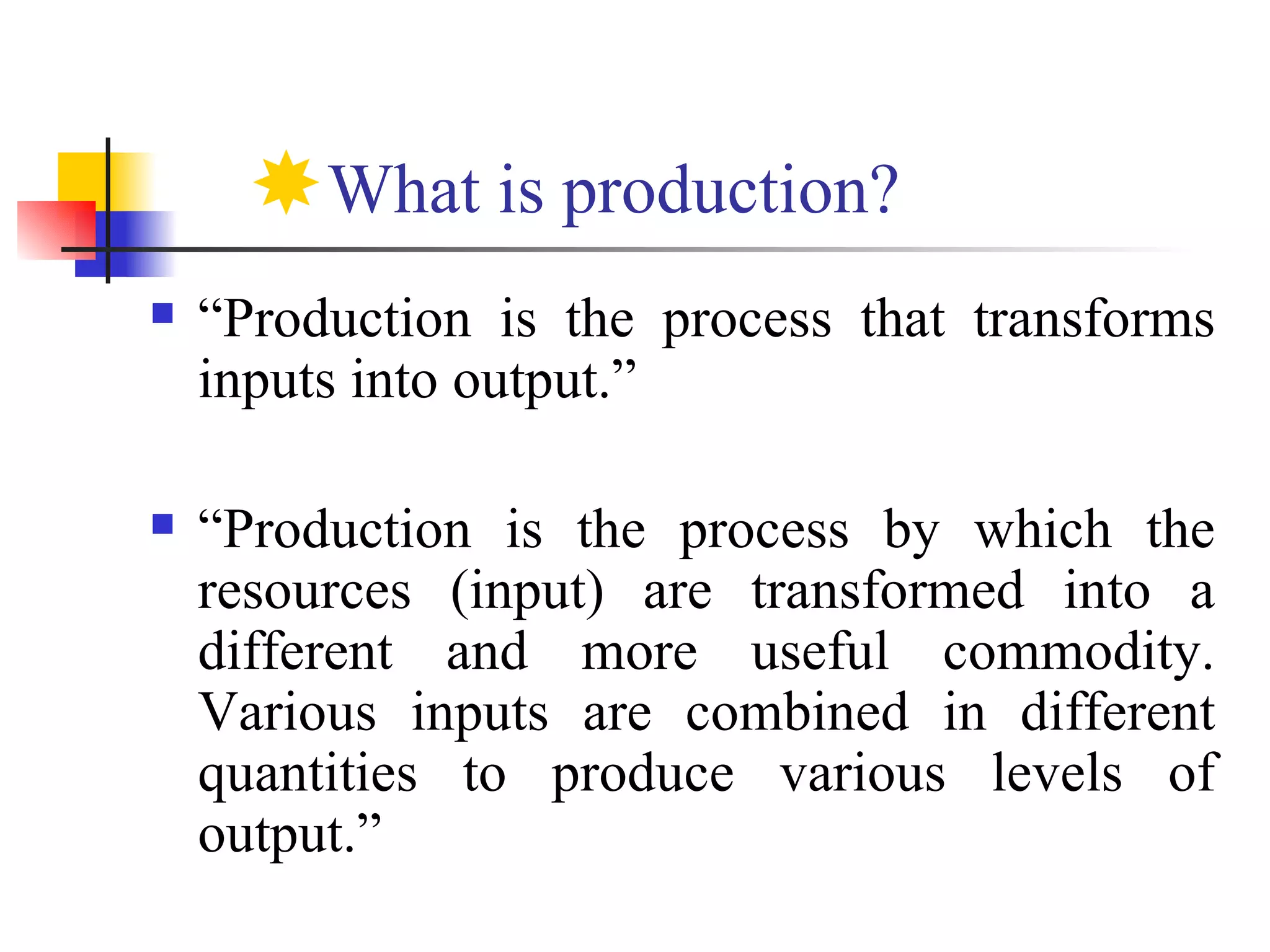
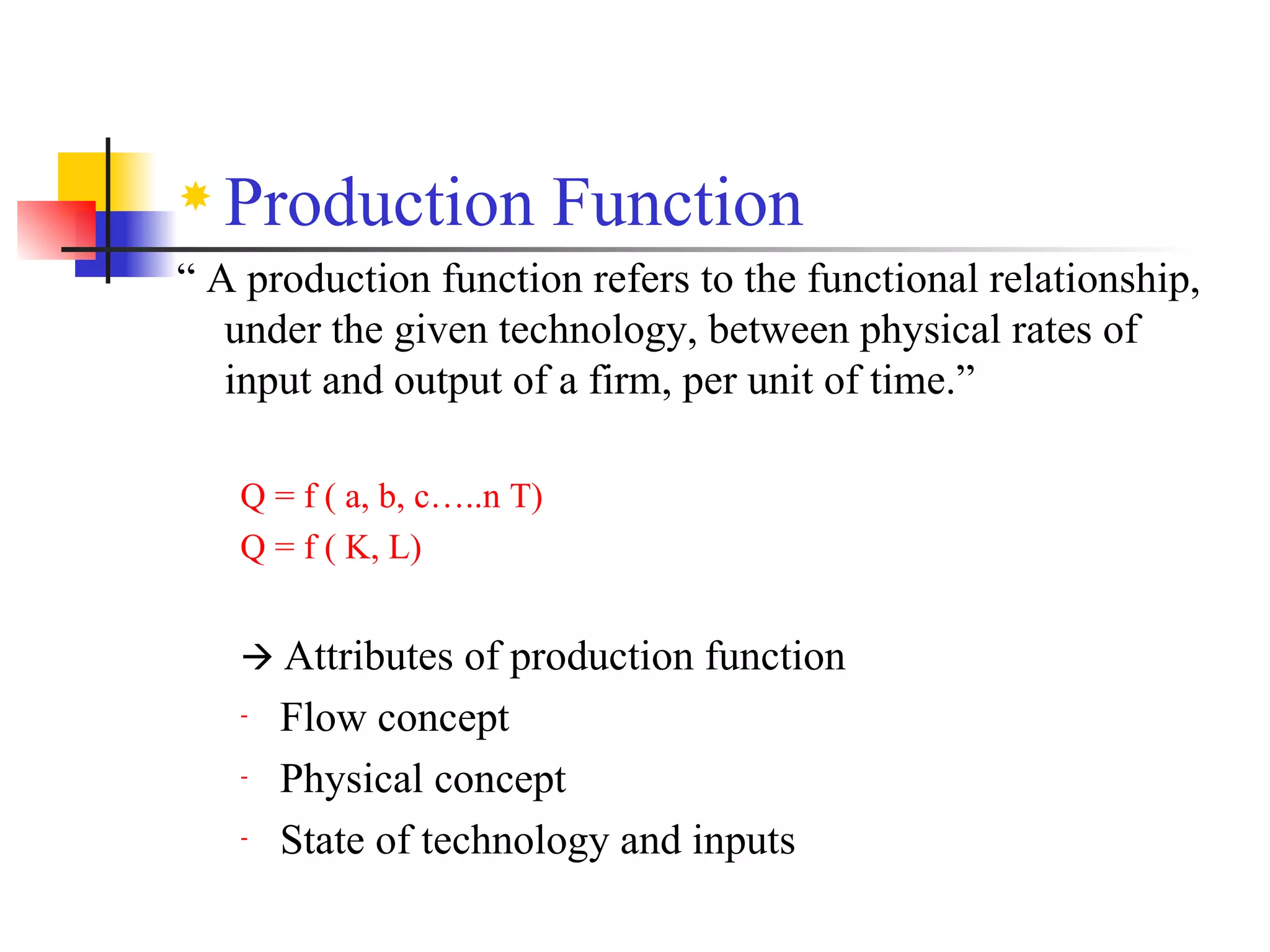
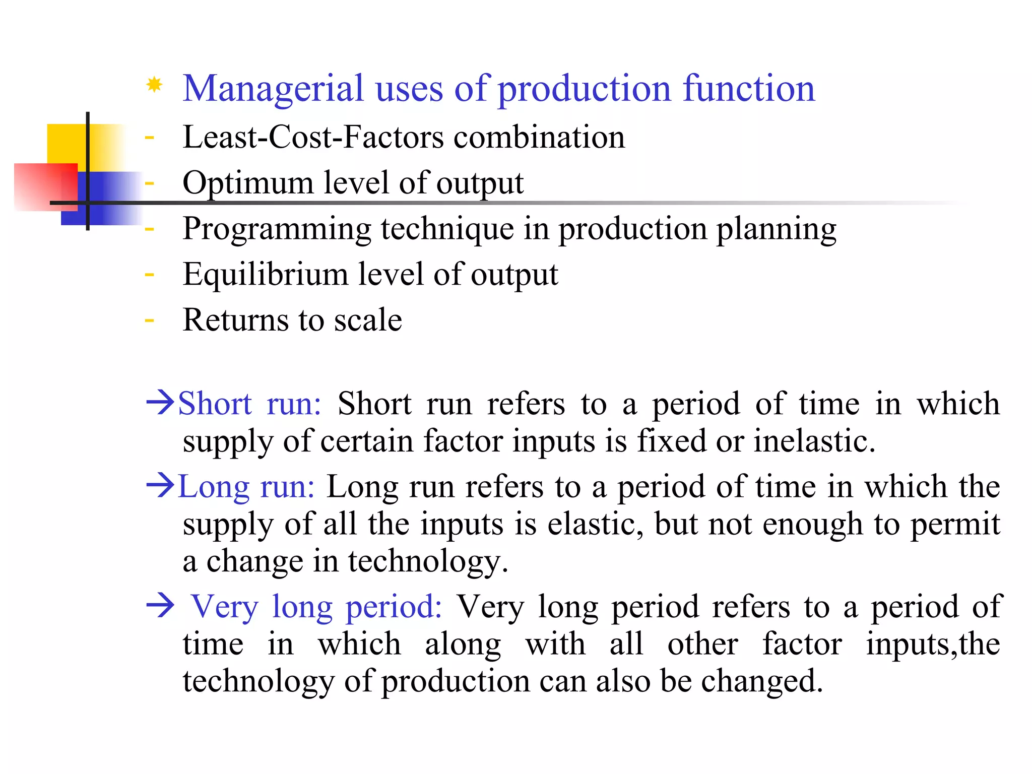
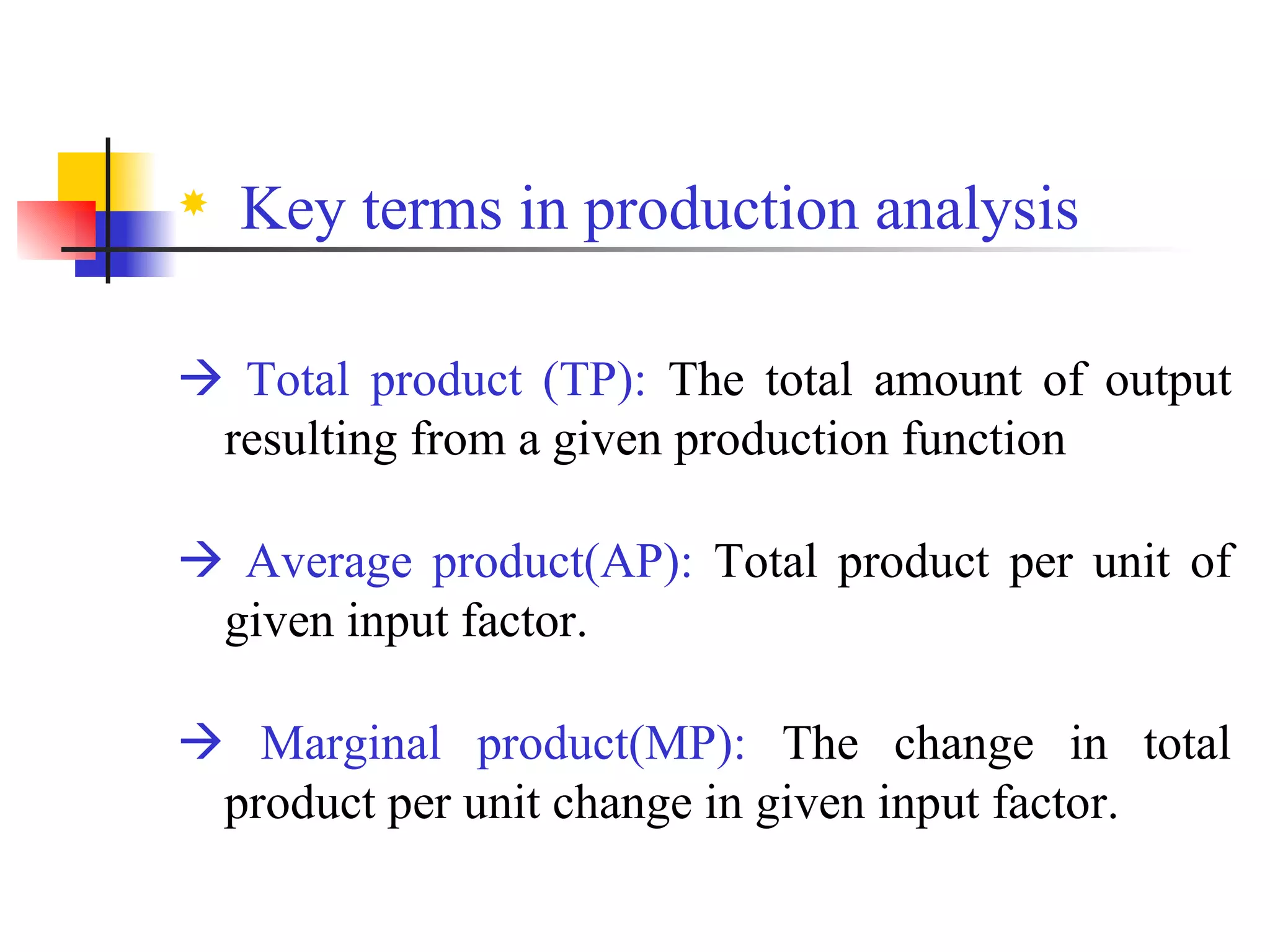
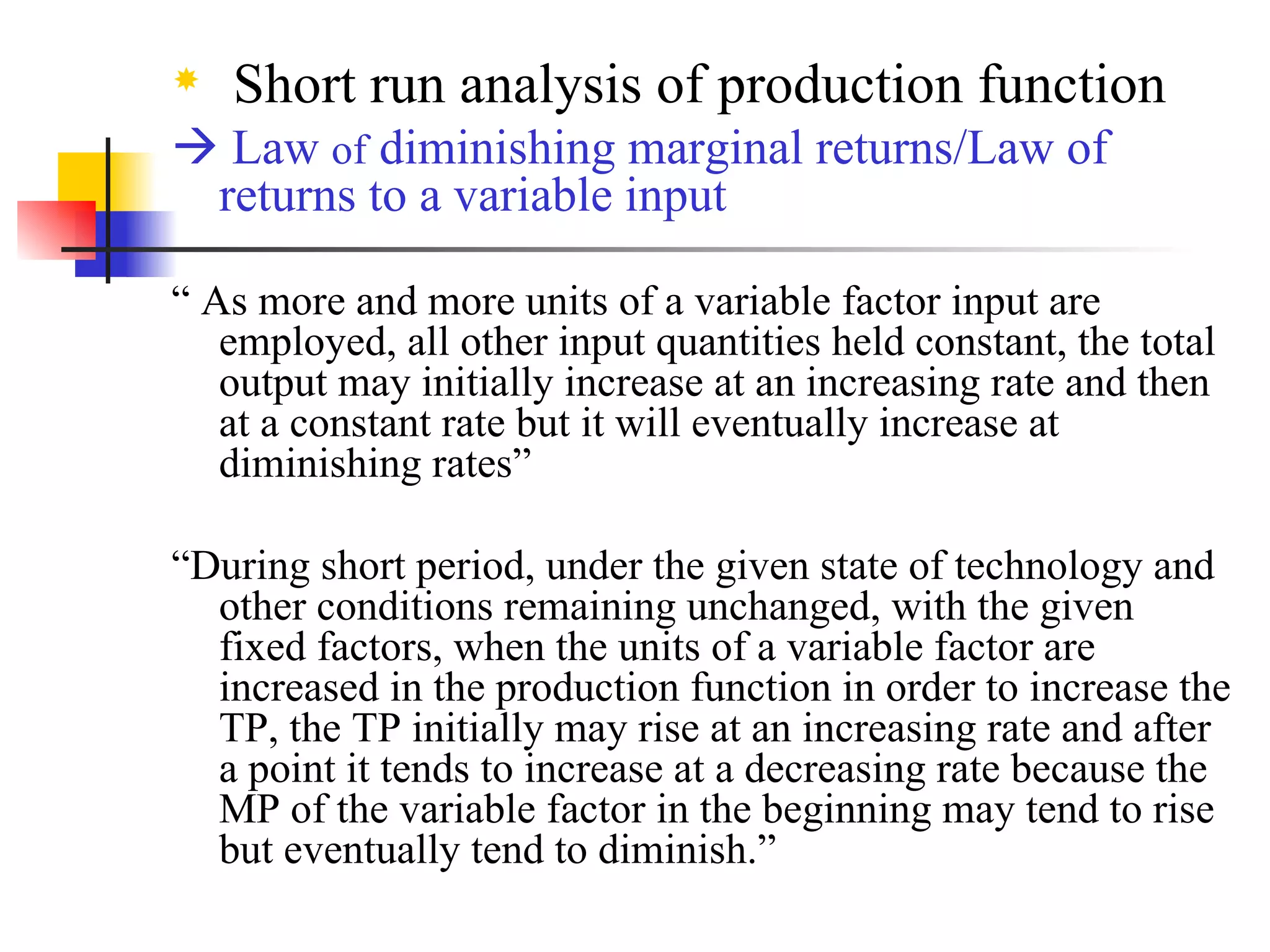
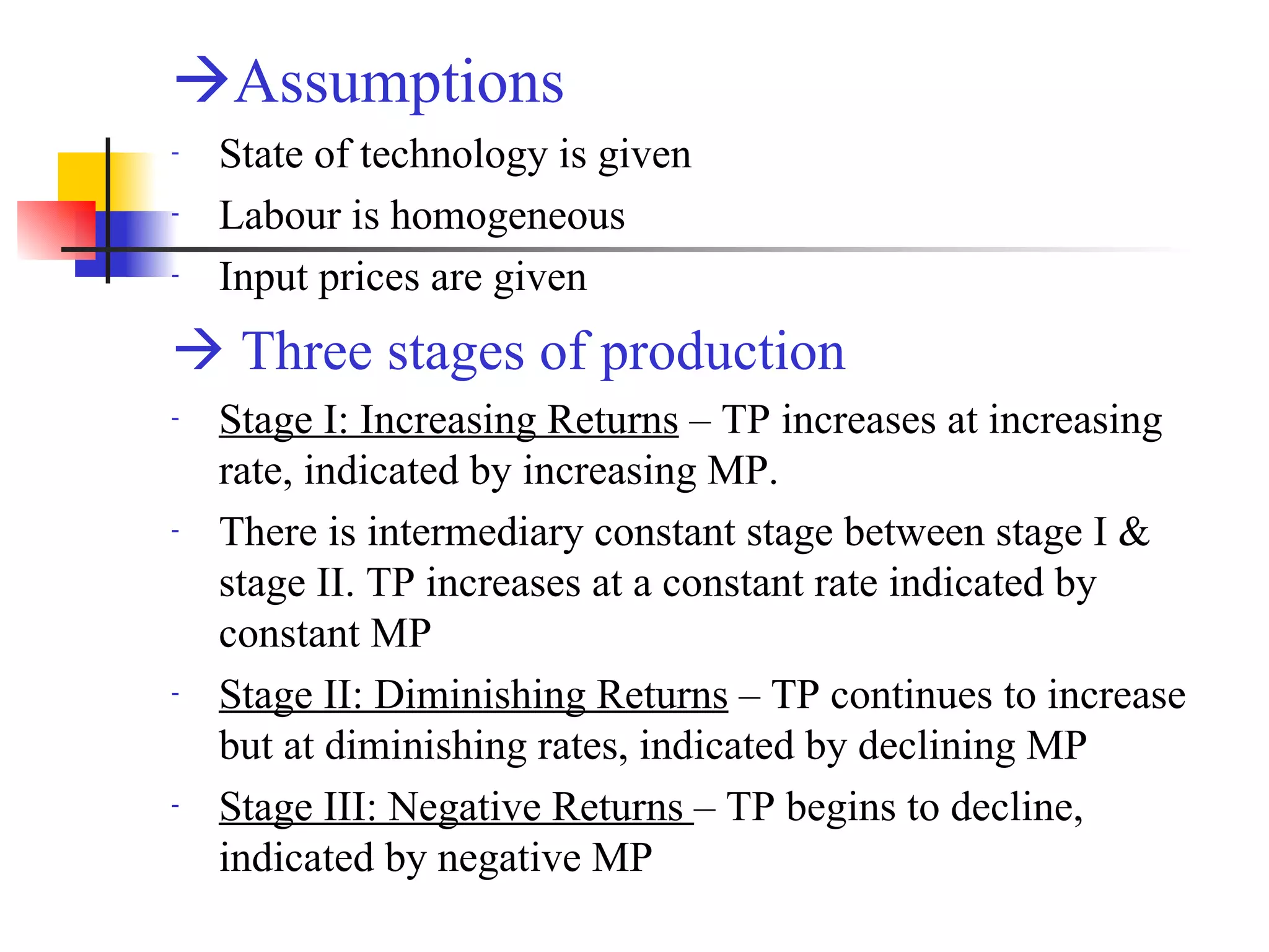
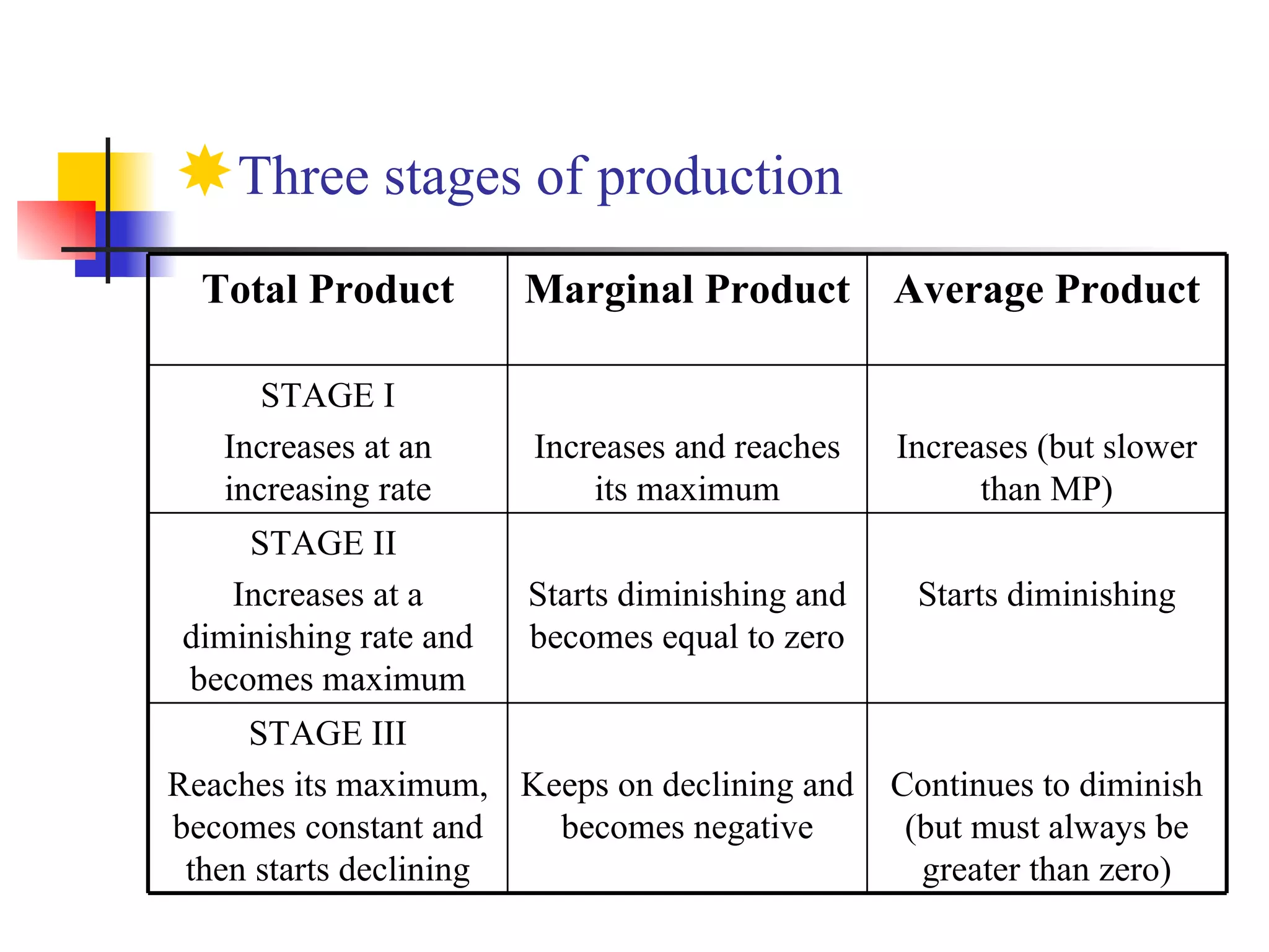
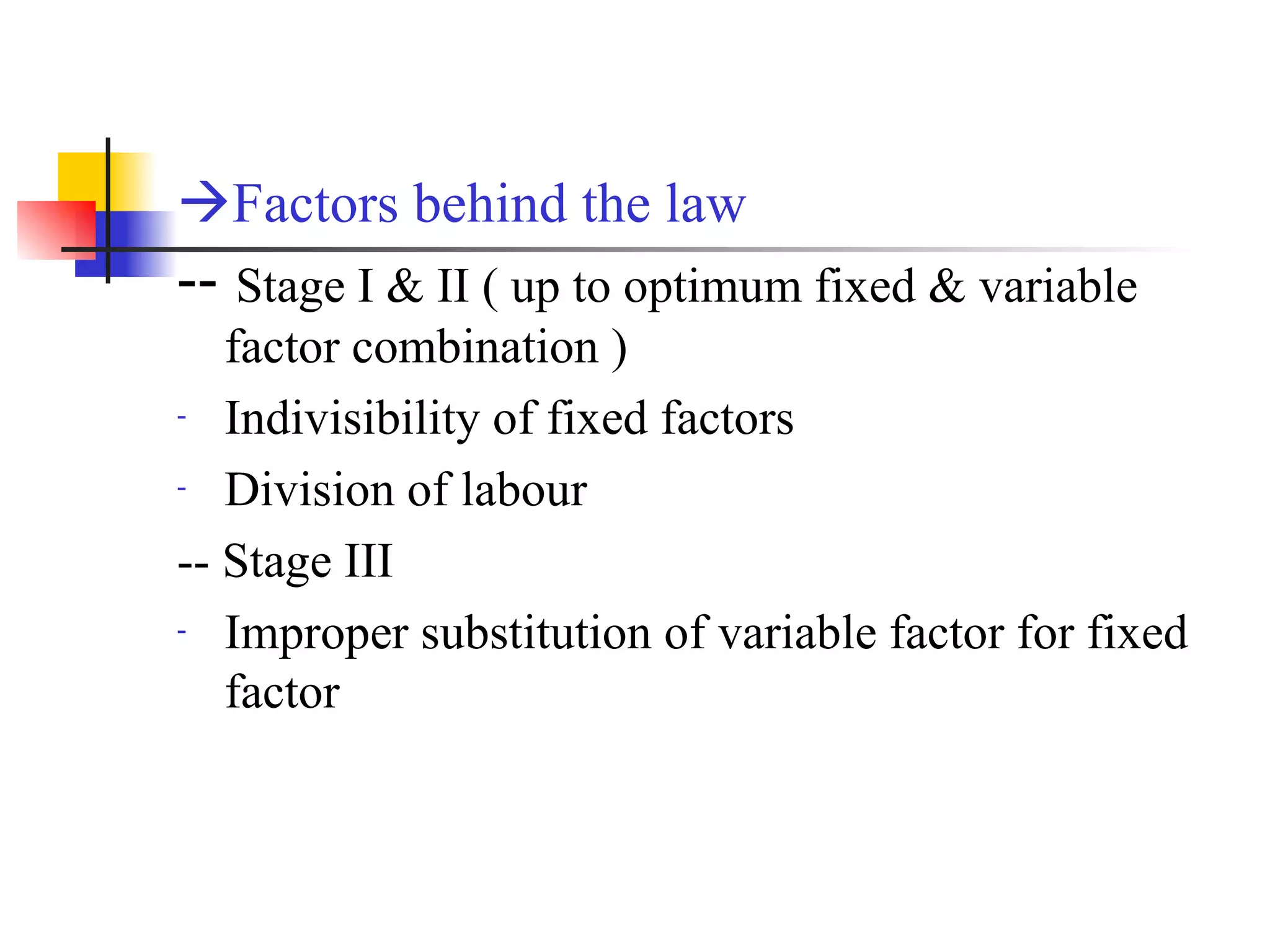
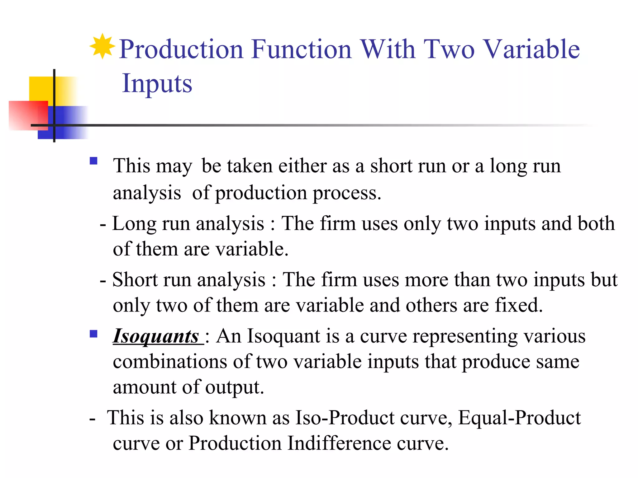
This document discusses key concepts related to production analysis including: 1. It defines production as the process of transforming inputs into outputs and describes a production function as the relationship between inputs and outputs. 2. It outlines short run, long run, and very long run periods and explains factors of production, total product, average product, and marginal product. 3. It describes the three stages of production - increasing, constant, and diminishing returns - and the law of diminishing marginal returns as it relates to a variable input factor.

1. PRODUCTION ANALYSIS

2. What is production? “ Production is the process that transforms inputs into output.” “ Production is the process by which the resources (input) are transformed into a different and more useful commodity. Various inputs are combined in different quantities to produce various levels of output.”

3. Production Function “ A production function refers to the functional relationship, under the given technology, between physical rates of input and output of a firm, per unit of time.” Q = f ( a, b, c…..n T) Q = f ( K, L)  Attributes of production function Flow concept Physical concept State of technology and inputs

4. Managerial uses of production function Least-Cost-Factors combination Optimum level of output Programming technique in production planning Equilibrium level of output Returns to scale  Short run: Short run refers to a period of time in which supply of certain factor inputs is fixed or inelastic.  Long run: Long run refers to a period of time in which the supply of all the inputs is elastic, but not enough to permit a change in technology.  Very long period: Very long period refers to a period of time in which along with all other factor inputs,the technology of production can also be changed.

5. Key terms in production analysis  Total product (TP): The total amount of output resulting from a given production function  Average product(AP): Total product per unit of given input factor.  Marginal product(MP): The change in total product per unit change in given input factor.

6. Short run analysis of production function  Law of diminishing marginal returns/Law of returns to a variable input “ As more and more units of a variable factor input are employed, all other input quantities held constant, the total output may initially increase at an increasing rate and then at a constant rate but it will eventually increase at diminishing rates” “ During short period, under the given state of technology and other conditions remaining unchanged, with the given fixed factors, when the units of a variable factor are increased in the production function in order to increase the TP, the TP initially may rise at an increasing rate and after a point it tends to increase at a decreasing rate because the MP of the variable factor in the beginning may tend to rise but eventually tend to diminish.”

7.  Assumptions State of technology is given Labour is homogeneous Input prices are given  Three stages of production Stage I: Increasing Returns – TP increases at increasing rate, indicated by increasing MP. There is intermediary constant stage between stage I & stage II. TP increases at a constant rate indicated by constant MP Stage II: Diminishing Returns – TP continues to increase but at diminishing rates, indicated by declining MP Stage III: Negative Returns – TP begins to decline, indicated by negative MP

8. Three stages of production Continues to diminish (but must always be greater than zero) Keeps on declining and becomes negative STAGE III Reaches its maximum, becomes constant and then starts declining Starts diminishing Starts diminishing and becomes equal to zero STAGE II Increases at a diminishing rate and becomes maximum Increases (but slower than MP) Increases and reaches its maximum STAGE I Increases at an increasing rate Average Product Marginal Product Total Product

9.  Factors behind the law -- Stage I & II ( up to optimum fixed & variable factor combination ) Indivisibility of fixed factors Division of labour -- Stage III Improper substitution of variable factor for fixed factor

10. Production Function With Two Variable Inputs This may be taken either as a short run or a long run analysis of production process. - Long run analysis : The firm uses only two inputs and both of them are variable. - Short run analysis : The firm uses more than two inputs but only two of them are variable and others are fixed. Isoquants : An Isoquant is a curve representing various combinations of two variable inputs that produce same amount of output. - This is also known as Iso-Product curve, Equal-Product curve or Production Indifference curve.

11. Properties of Isoquants It is downward sloping to the right (negatively inclined) It is convex to origin (Marginal Rate of Technical Substitution) Higher isoquant represents larger output No two isoquants intersect Types of Isoquants Linear isoquants – Perfect substitutability between factors of production Input-Output isoquants – Strict complimentarity / zero substitutability between input factors (fixed factor – proportion isoquants) Kinked isoquants – Limited substitutability between input factors Smooth, convex isoquants – Continuous substitutability over a certain range between the input factors

12.  Marginal Rate of Technical Substitution MRTS is the number of units of an input factor ( ex: K ) that a producer is willing to sacrifice for an additional unit of another input factor (ex: L) , so as to maintain the same level of output. (i.e., to remain on the same isoquant.)  Isoquant Map: A whole array of isoquants represented on a graph is called an isoquant map.  Economic Regions of Production – The ridge lines : The ranges over which the marginal products of the inputs are diminishing but positive. On a convex isoquant the MRTS decreases along the isoquant and can become zero. A zero MRTS determines the minimum quantity of an input which must be used to produce a given output. Beyond this point an additional employment of one input will necessitate employing additional units of other input. - A ridge line is the locus of points of isoquants where MP of input is zero.

13. Input Prices And Isocost Line ( budget line) Optimal Factor Combination - Production of given output at given cost - Production of maximum output with the given level of cost - Changes in firm’s resources and output: The Expansion path - Changes in factor prices and choice of technique

14. Laws of Returns to Scale The percentage increase in output when all inputs vary in the same proportion is known as returns to scale. It obviously relates to greater use of inputs maintaining the same technique of production.  Three Situations of Returns To Scale - Increasing Returns to Scale – Output increases by a greater proportion than the increase in input. - Constant Returns to Scale – Output increases in same proportion as increase in inputs. - Decreasing Returns to Scale – Output increases in a lesser proportion than the increase in input.

15. Economies of Large Scale Production Internal Economies of scale: They are those advantages which are open to an individual firm when its size expands. Labour Economies Technical Economies - Superior Technique - Increased Dimension - Linked Processes - By- products Managerial Economies Marketing or Commercial Economies Financial Economies Transport & Storage Economies Overhead Economies Economies of Vertical Integration Risk bearing Economies - Diversification of output - Diversification of market - Diversification of source of supply – Diversification of process of manufacturing

16. External Economies of scale: They are those benefits or advantages available to all the firms in the industry from outside, irrespective of their size and scale of operation, due to expansion of the industry size. Economies of Localisation / Concentration` Economies of Information Economies of Vertical Disintegration Economies of By- products Internal Diseconomies of scale:  Difficulties of management  Difficulties of Co-Ordination  Difficulties of Decision making  Increased risk  Labour Diseconomies  Scarcity of Factor Supplies  Financial difficulties  Market diseconomies External Diseconomies of scale: