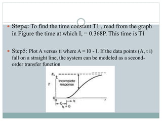
The document discusses process identification, which involves experimentally determining the dynamic behavior of industrial processes too complex to model using fundamental principles. Process identification provides models like process reaction curves from step inputs, frequency response diagrams from sinusoidal inputs, and pulse responses. These models are useful for control system design. The document specifically describes using a step test and semi-log plotting of the process reaction curve to identify the parameters of a second-order process model with transport lag, including the time constants T1 and T2 and the process gain Kp.

1. S U B M I T T E D B Y
RCS SIDDHARTH
1 5 1 FA 1 7 0 1 8
3 R D P E T R O L E U M E N G I N E E R I N G
An introduction to PROCESS
IDENTIFICATION

2. Introduction
 The processes used in our control systems have been described by transfer functions
that were derived by applying fundamental principles of physics and chemical
engineering (e.g., Newton’s law, material balance, heat transfer, fluid mechanics,
reaction kinetics, etc.) to well defined processes
 Many of the industrial processes to be controlled are too complex to be described by
the application of fundamental principles
 By means of experimental tests, one can identify the dynamical nature of such
processes and from the results obtain a process model which is at least satisfactory for
use in designing control systems

3.  The experimental determination of the dynamic behavior of a
process is called process identification
 Process identification provides several forms that are useful in
process control; some of these forms are
1. Process reaction curve (obtained by step input)
2. Frequency response diagram (obtained by sinusoidal input)
3. Pulse response (obtained by pulse input)

4.  In the case of the Z-N method, the procedure obtained one point on the open-
loop frequency response diagram when the ultimate gain was found. (This
point corresponds to a phase angle of - 180’ and a process gain of l/Kc , at the
cross-over frequency w,,.) In the case of the C-C method, the process
identification took the form of the process reaction curve
 Step Testing:- a step change in the input to a process produces a response,
which is called the process reaction curve
 The process reaction curve is an S-shaped curve. It is important that no
disturbances other than the test step enter the system during the test, otherwise
the transient will be corrupted by these uncontrolled disturbances and will be
unsuitable for use in deriving a process model

5.  For systems that produce an S-shaped process reaction
curve, a general model that can be fitted to the transient
is the following second-order with transport lag model:
 SEMI-LOG PLOT FOR MODELING. The transfer function
given by eqn can be obtained from a process reaction curve by a
graphical method in which the logarithm of the incomplete
response is plotted against time. In principle, this method can
extract from the process reaction curve the two time constants in
Eqn . The method, referred to as the semi-log plot method, is
outlined below. The method applies for T1 > T2.

6. Steps involved
 Step1:Determine (if transport lag is present) the time at which the process
reaction curve first departs from the time axis; this time is taken as the
transport lag Td
 Step2: From the process reaction curve , plot I versus t 1 on semi-log paper as
shown in Figure where Z is the fractional incomplete response and tl is the
shifted time starting at Td (i.e., t 1 = t - Td). I is defined by
 Bu is the ultimate value of Y
 Step3: Extend a tangent line through the data points at large values of figure.
Refer to this tangent line as I, and let the intersection of the tangent line with
the vertical axis at t 1 = 0 be called Z

7.  Step4: To find the time constant T1 , read from the graph
in Figure the time at which I, = 0.368P. This time is T1
 Step5: Plot A versus ti where A = I0 - I. If the data points (A, t i)
fall on a straight line, the system can be modeled as a second-
order transfer function

8.  with transport lag as given by Eqn with time constants T1 and T2. The
value of T2 is the time at which A = 0.368R where R is the intersection
of the line A with the vertical axis at ti = 0. If one does not get a straight
line when A is plotted against ti, the procedure can be extended to get
more first-order time constants, T3, T4, and so on; however, the data
must be very accurate for this method to be successful in identifying
more than two time constants. Usually the data scatter, especially at
large values of time, and one must be satisfied in drawing straight lines
through the scattered points.
 Step6: The process gain is simply Kp = Bu/M

12. References
 Process dynamics and control by Donald R
Coughnawor
 Thank-you
 For the book please mail me at
siddharthrcs@gmail.com and for queries you can
mail me