This paper presents a novel method for tuning PID controllers based on process step response and a damping optimum criterion. The method identifies parameters of an nth order lag (PTn) process model from the step response. This facilitates algebraic rules for adjusting closed-loop response speed and damping. The effectiveness of the proposed PTn parameter estimation and PID tuning is verified through simulations. The method provides a straightforward way to tune both closed-loop response damping and speed in relation to process dynamics for higher-order aperiodic processes.

1. Research Article
PID controller auto-tuning based on process step response
and damping optimum criterion
Danijel Pavković a,n
, Siniša Polak b
, Davor Zorc a,1
a
Faculty of Mechanical Engineering and Naval Architecture, University of Zagreb, I. Lučića 5, HR-10000 Zagreb, Croatia
b
INA-Oil Industry d.d. – Sisak Oil Refinery, Ante Kovačića 1, HR-44000 Sisak, Croatia
a r t i c l e i n f o
Article history:
Received 2 November 2012
Received in revised form
12 March 2013
Accepted 19 August 2013
Available online 12 September 2013
This paper was recommended for
publication by Dr. K.A. Hoo
Keywords:
PID controller
PTn process model
Damping optimum criterion
Identification
Auto-tuning control
a b s t r a c t
This paper presents a novel method of PID controller tuning suitable for higher-order aperiodic processes
and aimed at step response-based auto-tuning applications. The PID controller tuning is based on the
identification of so-called n-th order lag (PTn) process model and application of damping optimum
criterion, thus facilitating straightforward algebraic rules for the adjustment of both the closed-loop
response speed and damping. The PTn model identification is based on the process step response,
wherein the PTn model parameters are evaluated in a novel manner from the process step response
equivalent dead-time and lag time constant. The effectiveness of the proposed PTn model parameter
estimation procedure and the related damping optimum-based PID controller auto-tuning have been
verified by means of extensive computer simulations.
& 2013 ISA. Published by Elsevier Ltd. All rights reserved.
1. Introduction
Many industrial processes such as heat and fluid flow processes
are characterized by slow aperiodic dynamics (lag behavior)
and dead-time (transport delay), which are frequently modeled by
a control-oriented first-order plus dead-time (FOPDT) process model
[1,2], and are in a majority of cases still controlled by Proportional-
Integral-Derivative (PID) controllers [3–5]. Accordingly, the PID con-
troller auto-tuning still remains an interesting and propulsive R&D
field (see [6] and references therein), which has resulted in numerous
PID controller auto-tuning patents and commercial controller units
over the last several decades [7]. Among the patented and imple-
mented PID adaptation approaches the so-called analytical formula
methods, typically based on process open-loop (input step) or
closed-loop (limit-cycle) excitation test are usually preferred over
more complex tuning methods, such as those based on heuristic
rules, artificial intelligence and numerical optimization approaches.
In latter cases the closed-loop behavior is typically monitored with
the PID controller turned on, and PID controller adaptation is
performed in real-time without applying a dedicated test signal [8].
The conventional formula-based tuning methods, such as the
Ziegler–Nichols (ZN) tuning rules, even though still used in practical
applications due to their simplicity, may result in a relatively large
closed-loop step response overshoot and related weak response
damping [9,10]. The closed-loop damping issues have been tradi-
tionally addressed by using the Chien–Hrones–Reswick (CHR) ZN
rule modification based on the time-domain FOPDT process model
identification, while the so-called Kappa-Tau method has been
used for frequency response-based (i.e. ultimate point finding)
auto-tuning [11,12]. Some of the more recent efforts at ZN-rule
improvement have included controller parameters numerical opti-
mization for a wide range of FOPDT process model parameters
variations [5], and on-line adaptation of the PID controller propor-
tional gain [10].
In order to further improve the PID controller performance com-
pared to the above traditional tuning formulas, a wide range of process
excitation-based auto-tuning approaches has been proposed in the
literature over the last decade or so, which may be categorized as
Frequency response-based approaches aimed at (i) improved
gain and phase margin estimation [13–15], (ii) process model
identification based on closed-loop relay experiment in combi-
nation with internal model control (IMC) based controller
tuning for improved control-loop load disturbance rejection
[16], (iii) using a more general case of binary noise signal for
the process model frequency characteristic identification and
loop-shaping-based controller tuning for robust behavior [17],
(iv) use of Bode's integrals for improved closed-loop system
robustness [18], and (v) relay experiment with cascaded
Contents lists available at ScienceDirect
journal homepage: www.elsevier.com/locate/isatrans
ISA Transactions
0019-0578/$ - see front matter 2013 ISA. Published by Elsevier Ltd. All rights reserved.
http://dx.doi.org/10.1016/j.isatra.2013.08.011
n
Corresponding author. Tel.: þ385 1 6168 325; fax: þ385 1 6168 351.
E-mail addresses: danijel.pavkovic@fsb.hr (D. Pavković),
Sinisa.Polak@ina.hr (S. Polak), davor.zorc@fsb.hr (D. Zorc).
1
Tel.: þ385 1 6168 436; fax: þ385 1 6168 351.
ISA Transactions 53 (2014) 85–96

2. PI controller for load disturbance compensation and filtering
effect during process model identification [19]. For a rather
comprehensive review of relay-feedback frequency-domain
auto-tuning methods the reader is also referred to [20].
Time response approaches based on (i) process output multiple
integration and regression analysis in order to find the para-
meters of a second-order plus dead-time (SOPDT) process
model [21], (ii) multiple process step response integration to
find a general linear process model [22–24] combined with
the utilization of the so-called magnitude optimum criterion
in order to achieve well-damped closed-loop response, and
(iii) step-response identification of FOPDT model combined with
IMC tuning approach [25,26], or a robust loop-shaping controller
design (the so-called AMIGO method) [26,27].
Combined approaches wherein the time-domain and frequency-
domain process model identification is used, such as the
combined relay experimentþstep response identification of a
FOPDT process model [28], or a random signal-based process
excitation and SOPDT process model parameters estimation
and controller tuning based on zero-pole conditioning (cancel-
ing) [29].
However, in most of the above cases the PID controller tuning
was based on the relatively simple FOPDT (or SOPDT) process
model approximation with first-order Taylor or Padé dead-time
approximations used for the purpose of PID controller design,
which may not be accurate in the presence of more pronounced
higher-order process dynamics. In order to capture the higher-
order dynamics, while simultaneously having a relatively simple
dead-time-free process model formulation, an n-th order lag
process model (the so-called PTn model) can conveniently be
used, wherein analytical relationships between the PTn model and
FOPDT model parameters are typically given through the equiva-
lence of the process model step response flexion tangent (the so-
called Strejc method) [30,31]. By utilizing the PTn process model
as the basis for the control system design in [32], straightforward
analytical expressions have been derived for the PID controller
parameters based on the magnitude optimum criterion (see e.g.
[33] and references therein). The PTn model parameters have been
identified in [32] by using the so-called moment method (see e.g.
[30]), implemented through multiple time-weighted integrations
of the process output, thus avoiding the estimation of the process
step response flexion tangent slope (and related measurement
noise issues). Since the main advantage of the magnitude opti-
mum criterion is that it can assure a well-damped (over-damped)
closed-loop system response, this approach has also been pursued
for a wider class of linear process models in [22]. Further refine-
ments of the tuning method from [22] have included a filtering
term added to the PID controller transfer function to facilitate
relatively straightforward closed-loop response speed (response
time) tuning [23], and extending the PID controller with a
reference pre-filtering or weighting action to facilitate separate
closed-loop system tuning with respect to reference and external
disturbance [24].
Still, the aforementioned magnitude optimum-based PID con-
troller auto-tuning does not provide a straightforward way of closed-
loop damping adjustment, while the repetitive integration of process
output may result in an increased computational burden of the
PID controller auto-tuning algorithm, especially if application on a
relatively low-cost industrial controller is considered. Hence, a more
flexible pole-placement-like tuning method, as well as a simpler
process step response-based auto-tuning experiment (e.g. based on a
single integration of process step response) would result in a more
accommodating and less-demanding PID auto-tuner realization. To
this end, this paper proposes a PID controller tuning approach based
on the so-called damping optimum criterion [34,35] in combination
with the PTn process model formulation, which facilitates an
analytical and straightforward way of adjusting both the closed-
loop response damping and response speed with respect to process
dynamics. The estimation of PTn process model parameters is based
herein on the single integration of the process step response in
order to find the parameters of the basic FOPDT process model.
The simpler FOPDT model is then related to the equivalent dead-
time-free PTn model by using a higher-order Taylor expansion of the
dead-time (pure delay) dynamic term via simple analytical expres-
sions. The proposed PID controller tuning, the FOPDT and PTn
process model identification procedures and the resulting PID con-
troller auto-tuning algorithm is verified by means of extensive
computer simulations.
The paper is organized as follows. Section 2 presents the
analytical control system design procedure based on the damping
optimum criterion and the compact PTn aperiodic process model,
and illustrates the effectiveness of resulting closed-loop damping
and response speed tuning method. These results are also accom-
panied by the analysis of the closed-loop robustness with respect
to modeling uncertainties. The identification of PTn process model,
based on a single integration of the process output is described in
Section 3. The proposed identification procedure and the related
PID controller auto-tuning are thoroughly tested in Section 4 by
means of simulations. Concluding remarks are given in Section 5.
2. Control system design
This section presents the damping optimum criterion-based
tuning of the PID controller for the process model with aperiodic
step response dynamics, including the compact-form PTn process
model. The effectiveness of the proposed PID controller tuning
procedure, including the closed-loop damping tuning is illustrated
by means of simulations.
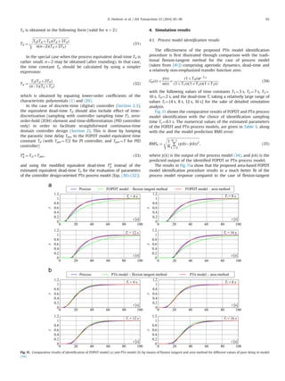
2.1. Control system structure
The structure of the linear control system comprising a mod-
ified PID feedback controller (the so-called IþPD controller, [41])
is shown in Fig. 1. In comparison with the traditional PID controller
where the proportional (P), integral (I), and derivative (D) terms
are placed into the path of the control error e, the proportional
and derivative terms of the modified PID controller act upon
the measured process output y only (Fig. 1). By opting to use the
modified PID controller structure which does not introduce addi-
tional controller zeros in the closed-loop transfer function, the
desired closed-loop system behavior can be achieved with respect
to the external disturbance w, while also avoiding the potentially
excessive control effort related to sudden reference yR changes or
“noisy” reference. Since the proposed control system design does
not introduce additional closed-loop zeros due to controller PþD
action, the proposed approach also results in relatively simple
Fig. 1. Block diagram of control system with modified PID controller.
D. Pavković et al. / ISA Transactions 53 (2014) 85–9686

3. and straightforward PID controller tuning rules (see Section 2.2).
Should the traditional PID controller structure be preferred, or the
reference and disturbance behavior of the closed-loop system be
tuned independently, somewhat more complex (two-step) tuning
approaches may be required, such as those presented in Refs. [24,36],
wherein the magnitude optimum-based tuning has been proposed to
separately tune the closed-loop system response with respect to
reference.
Note that in order to avoid relatively large step response
overshoots in the large-signal operating mode (so-called integra-
tor windup problem), the controller integral term should be
saturated when controller output saturation is performed
(Fig. 1), e.g. by using the so-called reset-integrator method [37].
It is assumed that the process is characterized by relatively
slow aperiodic dynamics (no step response overshoot or tran-
sient oscillations), which can be approximated by the n-th order
aperiodic process model with a single time constant Tp (the
so-called PTn model) [30–32], given in the following compact
transfer function form:
GpðsÞ ¼
yðsÞ
uðsÞ
¼
Kp
ð1þTpsÞn ¼
Kp
1þa1sþa2s2 þ⋯ansn
; ð1Þ
where Kp is the PTn model gain, nZ2 is the process order, and
the parameters of the process model characteristic polynomial am
(m¼1… n) are given by
am ¼
n
m
Tm
p ¼
n!
m!ðnÀmÞ!
Tm
p : ð2Þ
2.2. PID controller tuning
The PID controller tuning procedure is based on the damping
optimum (or double ratios) criterion [34,35]. This is a pole-
placement-like analytical method of design of linear continuous-
time closed-loop systems with a full or reduced-order controller,
which results in straightforward analytical relations between
the controller parameters, the parameters of the process model,
and desired level of response damping via characteristic design-
specific parameters. Even though somewhat less well known than
the magnitude optimum criterion [33], the damping optimum
criterion has found application in those control systems where the
closed-loop damping needs to be tuned in a precise and straight-
forward manner (e.g. in electrical servodrives with emphasized
transmission compliance effects, see [38–40]).
The tuning procedure starts with the transfer function of
the closed-loop control system in Fig. 1 assuming idealized PID
controller (typically, the derivative filter time constant Tν5TD, so it
may be neglected):
GcðsÞ ¼
yðsÞ
yRðsÞ
¼ 1= 1þ
ð1þKRKpÞTIs
KRKp
þ
ðKRKpTD þa1ÞTIs2
KRKp
þ
a2TIs3
KRKp
þ
a3TIs4
KRKp
þ⋯þ
anTIsn þ1
KRKp
: ð3Þ
The characteristic polynomial of the closed-loop system (3) can
be rewritten in terms of the damping optimum criterion in the
following form:
GcðsÞ ¼
1
AcðsÞ
¼
1
1þTesþD2T2
e s2 þD3D2
2T3
e s3⋯þDlD2
lÀ1 U U UDlÀ1
2 Tl
esl
;
ð4Þ
where Te is the equivalent time constant of the overall closed-loop
system, D2, D3, …, Dl are the so-called damping optimum char-
acteristic ratios, and l is the closed-loop system order (l¼nþ1 in
the case of PID controller, cf. (3)).
When all characteristic ratios are set to the so-called “optimal”
values D2¼D3¼…¼Dl¼0.5 (e.g. by applying a full-order controller),
the closed-loop system of any order l has a quasi-aperiodic step
response characterized by an overshoot of approximately 6% (thus
resembling a second-order system with damping ratio ζ¼0.707)
and the approximate settling time of 1.8–2.1Te, as illustrated in
Fig. 3a. This particular closed-loop tuning may be regarded as
optimal in those cases where small overshoot and related well-
damped behavior are critical, such as in controlled electrical drives
and related servodrive control applications. By choosing larger Te
value, the control system robustness is improved and the noise
sensitivity is decreased (i.e. bandwidth ΩBW$1/Te), but, in turn,
a slower response and less efficient disturbance rejection are
obtained. For a reduced-order controller with the number of free
parameters equal to r, only the dominant characteristic ratios
D2,…, Dr þ1 should be set to desired values. In this case, however,
the non-dominant characteristic ratios (corresponding to non-
dominant high-frequency closed-loop poles) cannot be adjusted
arbitrarily, so their effect to closed-loop damping should be
analyzed separately. In general, the response damping is adjusted
through varying the characteristic ratios D2, D3, … Dl, wherein the
damping of dominant closed-loop dynamics (i.e. the dominant
closed-loop poles damping ratio) is primarily influenced by the
most dominant characteristic ratio D2. By reducing the character-
istic ratio D2 to approximately 0.35 the fastest (boundary) aper-
iodic step response without overshoot is obtained. On the other
hand, if D2 is increased above 0.5 the closed-loop system response
damping decreases (see Fig. 3b).
The PID controller (r¼3) can arbitrarily adjust only the closed-
loop characteristic ratios D2, D3 and D4. Hence, the analytical
expressions for PID controller proportional gain KR, integral
time constant TI, and derivative time constant TD are obtained by
equating lower-order coefficients of the characteristic polynomial
in (3) with the coefficients of the characteristic polynomial (4) up
to s4
, which after some manipulation and rearranging yields the
following relatively simple analytical expressions:
KR ¼
1
Kp
nðnÀ1ÞT2
p
2D2
2D3T2
e
À1
!
; ð5Þ
TI ¼ 1À
2D2
2D3T2
e
nðnÀ1ÞT2
p
!
Te; ð6Þ
TD ¼ D2TeTpn
ðnÀ1ÞTpÀ2D2D3Te
nðnÀ1ÞT2
pÀ2D2
2D3T2
e
; ð7Þ
with the closed-loop equivalent time constant Te given as follows
(valid for n42):
Te ¼
ðnÀ2ÞTp
3D2D3D4
ð8Þ
Fig. 2. Block diagram of discrete-time PID controller with zero-order-hold element
at controller output.
D. Pavković et al. / ISA Transactions 53 (2014) 85–96 87

4. Similarly, in the case of PI controller (TD¼0), only the closed-
loop characteristic ratios D2, D3 can be tuned, so the design is
based on the coefficients of the characteristic polynomial (4)
up to s3
:
KR ¼
1
Kp
nTp
D2Te
À1
; ð9Þ
TI ¼ 1À
D2Te
nTp
Te; ð10Þ
while the equivalent time constant Te is now given by (valid for
n41):
Te ¼
ðnÀ1ÞTp
2D2D3
ð11Þ
The above expressions indicate that the PID controller para-
meters KR, TI and TD are directly influenced by the dominant
characteristic ratios D2 and D3, while the non-dominant character-
istic ratio D4 only affects the closed-loop equivalent time constant
Te. Similarly, the simpler PI controller tuning is directly affected by
the most dominant characteristic ratio D2, while the closed-loop
equivalent time constant Te directly depends on the less-dominant
characteristic ratio D3 value. Thus, it appears that the closed-
loop response speed and dominant-mode damping tuning can be
effectively decoupled, because the damping of the dominant
closed-loop system modes is primarily determined by the choice
of the most dominant characteristic ratio D2, while the response
speed primarily depends on the closed-loop equivalent time
constant Te.
It should be noted, however, that for the cases of first-order lag
model (n¼1) or a second-order model (n¼2), the above expressions
for PI and PID controller parameters (5)–(11) are characterized by a
singularity. Namely, in those particular cases the PI and PID con-
trollers may be considered as respective full-order controllers, which
results in an arbitrary choice for the equivalent time constant Te
(see discussion above). For those particular cases, the expressions
for controller parameters are listed in Table 1. Note, however, that
a too small Te choice would result in significant control efforts
and controller output saturation during reference or disturbance
response transients. Moreover, the closed-loop system noise
sensitivity (i.e. bandwidth ΩBW) is directly related to the Te value
(ΩBW$1/Te), so the closed-loop equivalent time constant should also
have to be chosen such as to achieve favorable suppression of the
measurement noise and related chattering effects in the controller
output (manipulated variable) u.
Since PI and PID controller are of a relatively low order, they
cannot arbitrarily set the higher, non-dominant characteristic
ratios in the case of a high-order closed-loop system, so the effect
of high-order closed-loop modes is analyzed herein in terms of
damping optimum criterion and closed-loop system root-locus
plots. By combining Eqs. (3) and (4), and using the expression (2)
for the process parameters am, the higher-order characteristic
ratios Dm (where m43 for PI controller, and m44 for PID
controller) can be expressed by the following simple relation:
Dm ¼
ðnÀmþ1ÞðmÀ1Þ
ðnÀmþ2Þm
¼ 1À
1
nÀmþ2
1À
1
m
: ð12Þ
These characteristic ratios should be close to 0.5 for higher-order
characteristic ratios (i.e. higher m):
lim
m-n
Dm ¼
1
2
1À
1
n
; ð13Þ
which points out to well-damped nature of high-frequency modes.
Fig. 4 shows the root-locus plots of closed-loop systems with
PI and PID controller (normalized with respect to the PTn model
time constant Tp), for a wide range of process model orders n. The
root-locus plots confirm that the higher-order closed-loop modes
are indeed well-damped, i.e. the less-dominant closed-loop poles
(corresponding to higher-frequency modes) are all characterized
by damping ratio ζE0.707.
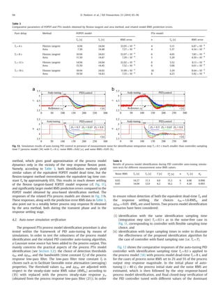
2.3. Discrete-time PID controller implementation
In the case when the PID controller is implemented as a discrete-
time controller (Fig. 2), the design procedure can still be carried out in
the continuous-time domain if the influence of the time-discretization
(sampling) is adequately taken into account. The series connection of
the sampler and the zero-order hold (ZOH):
GsEðsÞ ¼
1
T
GEðsÞ ¼
1ÀeÀsT
Ts
; ð14Þ
corresponds to a T/2 delay (T is the sampling time) cascaded to the
process [41].
The time-differentiation effective delay T/2 of the PID controller
derivative term (z–1)/(Tz) [42] can be added to the T/2 time delay
due to the sampler and time-discretization, thus resulting in the
overall parasitic time delay Tpar ¼T. This equivalent parasitic time
delay can then be lumped with the process equivalent dead-time
Td (see e.g. [41]), obtained by the FOPDT model identification
procedure described in Section 3.
Fig. 3. Step response of prototype system tuned according to damping optimum (a) and illustration of closed-loop damping variation through dominant characteristic ratio
D2 (b).
Table 1
PI and PID controller parameters for first-order and
second-order process model formulations.
Controller (process model order)
PI (n¼1) PID (n¼2)
KR ¼
1
Kp
Tp
D2Te
À1
KR ¼
1
Kp
T2
p
D3D2
2T2
e
À1
!
TI ¼ Te 1À
D2Te
Tp
TI ¼ Te 1À
D3D2
2T2
e
T2
p
!
–
TD ¼ Tp
Tp
D3D2Te
À2
D. Pavković et al. / ISA Transactions 53 (2014) 85–9688

5. The sampling time choice (where possible) represents a trade-off
between the controller performance and its computational burden
and measurement noise issues. For processes with notable response
pure delay, the sampling time T is typically chosen with respect to
the equivalent process dead-time Td and lag time constant Ta of the
process step response (see Section 3) as follows [41]
T %
ð0:35À1:2ÞTd; 0:1rTd=Ta r1;
ð0:22À0:35ÞTd; 1rTd=Ta r10:
(
ð15Þ
Note, however, that in the case of commercial PID controller
modules (see e.g. [12]), or PLC control hardware configuration
utilizing intelligent sensors (with internal signal processing fea-
tures and typically fixed data transfer rate), the controller sam-
pling rate may be pre-determined by the control hardware
internal design. Therefore, in those cases the sampling time may
not be regarded as the controller design parameter chosen
relatively freely according to Eq. (15), but rather as a fixed
parameter which needs to be taken into account during the
controller design (tuning), as explained earlier.
2.4. Simulation verification of controller tuning
The properties of the proposed PI and PID controller tuning
approach are illustrated in Figs. 5 and 6 by simulation results.
Fig. 5 shows the comparative simulation responses of continuous-
time closed-loop systems with PI and PID controllers tuned for a
damping-wise conservative, quasi-aperiodic response (D2¼D3¼
D4¼0.5) and PTn process models characterized by Kp¼1, Tp¼10 s
and model orders in the range n¼3–5. The results show that the
proposed controller tuning with all dominant characteristic ratios
set to 0.5 indeed results in well-damped control system responses
with respect to both the reference yR and input disturbance w
step changes, characterized by approximately 6% response overshoot.
As expected, the closed-loop equivalent time constant Te, and, hence,
the control system response time increases with the process order n
(cf. Eqs. (8) and (11)). Note also that for low process model order
n¼3, the PID controller results in a much faster step reference
response and notably improved disturbance rejection compared to PI
controller, because in that particular case the PID controller design
yields a notably smaller value of the closed-loop equivalent time
constant (Te¼26.7 s) compared to PI controller (Te¼40 s). However,
as the process model order increases, the aforementioned discre-
pancy becomes smaller, and the PID controller yields control system
performance similar to simpler PI controller.
The closed-loop step responses in Fig. 6 illustrate the effects of
varying the closed-loop equivalent time constant Te according to
Eqs. (8) and (11), wherein Te adjustment reflects in the change
of the less-dominant characteristic ratios (D3 in the case of
PI controller, and D4 in the case of PID controller). If the closed-
loop equivalent time constant Te is increased above the design
value according to (8) and (11), this results in a slower closed-
loop response. As expected, by decreasing the closed-loop equiva-
lent time constant Te below these values, the response speed
Fig. 4. Normalized root-locus plots of optimally-tuned closed loop-systems with PI controller (a) and PID controller (b) for different PTn process model orders.
Fig. 5. Reference and disturbance step responses of control systems with PI controller (a) and PID controller (b) for different orders of PTn process model.
D. Pavković et al. / ISA Transactions 53 (2014) 85–96 89

6. can indeed be increased. However, this corresponds to effective
increase of less-dominant characteristic ratios (D3 or D4), and
related lower damping of the less-dominant (higher-frequency)
closed-loop modes.
2.5. Robustness analysis
The effects of PTn process model uncertainty to control system
robustness (i.e. damping of dominant closed-loop modes) have
been analyzed by means of root-locus plots and simulations for
two choices of the most dominant characteristic ratio D2 used in
PI/PID controller design (with D3, D4 ¼0.5), and a fourth-order PTn
process model formulation. Note that the results of dominant
mode damping analysis should generally be valid for a wide range
of PTn model orders n, because the damping of higher-order
modes is not affected by controller tuning or by the value of PTn
model time constant Tp (see results in Fig. 4 and the related
discussion in Section 2.2). The modeling uncertainty effects are
examined for the case of relatively large 725% variation of the
PTn model time constant Tp, reflected through its relative
error εTp¼Tp/Tpn À1 (where Tpn is the nominal PTn model time
constant used in PI/PID controller design and Tp is the actual time
constant value).
The normalized root locus plots in Fig. 7 show that for the case
of PI and PID controller tuned for a damping-wise conservative
behavior (D2 ¼0.5), the dominant conjugate-complex closed-loop
pole pair for εTP¼ À25% (Tp oTpn) is shifted towards the area of
higher damping (ζ40.707), while in the case of Tp larger then
nominal (εTP¼ þ25%), the aforementioned pole pair remains fairly
well-damped (ζE0.5). On the other hand, for the case of PI and
PID controller tuned less-conservatively, i.e. with higher D2 value
(D2 ¼0.8) corresponding to weaker damping (and faster response),
the dominant closed-loop poles are shifted towards the area of
somewhat weaker damping (0.5oζo0.25), which may still be
acceptable for process control applications favoring fast response
over closed-loop damping considerations [12].
The root-locus results in Fig. 7 are also corroborated by the
closed-loop system simulation results shown in Fig. 8 (with the
time responses also normalized with respect to time constant Tp).
The results show that for the case of damping-wise conservative
tuning (D2 ¼0.5) the closed-loop responses are indeed rather well-
damped, with notably slower (aperiodic) response without over-
shoot occurring for the case of time constant Tp smaller nominal
(εTp¼ À25%). By tuning the PI or PID controller less conservatively
(D2 ¼0.8), faster closed-loop responses can be obtained, but this
is indeed paid for by somewhat more oscillatory reference step
response.
Based on the above results, the proposed method apparently
ensures a favorable level of closed-loop system robustness in the
presence of rather large process model uncertainty even for the
Fig. 7. Normalized root-locus plots of differently-tuned closed loop-systems with PI controller (a) and PID controller (b) for 725% variations of PTn process model time
constant Tp (n¼4).
Fig. 6. Comparative control systems responses for PI controller (a) and PID controller (b) tuned with D2¼0.5 and different values of closed-loop equivalent time constant Te
(PTn process model, Kp ¼1, Tp ¼10 s, n¼4).
D. Pavković et al. / ISA Transactions 53 (2014) 85–9690

7. case of damping-wise less-conservative controller tuning choice.
Still, the choice of the main PI/PID controller tuning parameter
(i.e. characteristic ratio D2) is obviously a trade-off between the
closed-loop response speed performance, and the prescribed
(desired) lower bound of the dominant closed-loop modes damp-
ing ratio.
3. Process model identification
This section presents the estimation of aperiodic process model
parameters based on the process step response integration and
identification of equivalent FOPDT process model (the so-called area
method). The proposed process model identification approach is
compared to the traditional flexion tangent method of estimation of
FOPDT and PTn process model parameters, and is used as a basis for a
PID controller auto-tuning algorithm.
3.1. Step response flexion tangent approach
Traditionally, processes characterized by aperiodic step response
and notable initial delay (equivalent dead-time) are modeled by using
the equivalent first-order plus dead-time (FOPDT) process model:
GpðsÞ ¼
KpeÀsTd
1þTas
ð16Þ
where the equivalent dead-time Td and the time constant Ta of the
first-order lag term are typically determined by the so-called flexion-
tangent approach [31], as illustrated in Fig. 9. In order to obtain a more
convenient dead-time-free process model (suitable for PI/PID control-
ler tuning described in Section 2), the FOPDT process model can be
directly related to the more accurate PTn process model (1), char-
acterized by the same response slope (time-derivative) at the flexion
point (the so-called Strejc method [30]). The relationships between the
FOPDT model and PTn process model parameters are given by
Td
Ta
¼ eð1ÀnÞ ðnÀ1Þn
ðnÀ1Þ!
þ ∑
nÀ1
m ¼ 0
ðnÀ1Þm
m!
À1; ð17Þ
Tp
Ta
¼
ðnÀ1ÞnÀ1
ðnÀ1Þ!
eð1ÀnÞ
; ð18Þ
with the results of numerical evaluation of above equations for n¼
2–10 shown in Table 2.
Note, however, that the accuracy of thus obtained FOPDT model
is favorable only over the equivalent dead-time interval Td and in
the vicinity of the process response flexion point, while the later
part of the process transient response is captured less accurately
(see Fig. 9).
3.2. FOPDT process model identification based on step
response integration
Since the above flexion tangent identification method may
be sensitive to process measurement noise (when finding the
response time-derivative maximum point), the FOPDT model may
instead be identified based on the step response time-integral
(area) method [43], shown in Fig. 10. In this approach, the pro-
cess step response time integral is related to the FOPDT model
response in the following manner:
I1 ¼
Z Tf in
0
ðyðtÞÀy1Þdt %
Z Tf in
0
ðy2Ày1Þ½1ÀeÀðtÀTdÞ=Ta
Šdt
¼ ðy2Ày1Þ Tf inÀTdÀTa þTaeÀðTf inÀTdÞ=Ta
h i
; ð19Þ
If the identification interval Tfin is larger than 5TaþTd (the
steady-state condition), the exponential term on the rightmost
side of Eq. (19) becomes negligible (i.e. it is less than 0.01), and the
following relationship is valid:
Ta ¼ Tf inÀTdÀ
I1
y2Ày1
; ð20Þ
The process model equivalent dead-time Td can be determined
by means of a simple threshold crossing logic, as illustrated in
Fig. 10, while the process model gain Kp is estimated based on the
Fig. 8. Normalized simulation responses of differently-tuned closed loop-systems with PI controller (a) and PID controller (b) for 725% variations of PTn process model time
constant Tp (n¼4).
Fig. 9. Illustration of identification of FOPDT model based on the step response
flexion tangent approach.
D. Pavković et al. / ISA Transactions 53 (2014) 85–96 91

8. process steady-states y2 and y1 and the input step magnitude Δu
as Kp¼(y2 Ày1)/Δu (see Fig. 9).
In practical applications, the above FOPDT process model
identification procedure (implemented as a discrete-time algo-
rithm) would also need to include the following features:
Process output averaging (low-pass filtering) required to correctly
estimate the process initial state y1 and the step response steady-
state y2 in the presence of process output measurement noise.
This can be facilitated by using a simple first-order low-pass term
(filter):
yf ðkTsÞ ¼ af yf ðkTsÀTsÞþð1Àaf ÞyðkTsÞ; ð21Þ
where Ts is the process response sampling time, and the discrete-
time filter coefficient af is related to the filter equivalent time
constant Tf as af¼exp(ÀTs/Tf). The same filtered output signal
can conveniently be used for the detection of process response
equivalent dead-time. Note that in that case the dead-time value
Tdf obtained from the filtered process output should be adjusted
with respect to the low-pass filter equivalent delay (correspond-
ing to filter time constant Tf):
Td ¼ Tdf ÀTf : ð22Þ
Finally, the low-pass filter can also be used to detect the process
response settling after the step transient by monitoring the time-
difference of the low-pass filtered process output Δyf(kTs)¼
yf(kTs)Àyf(kTs–Ts), where the steady-state could be detected by
simple threshold logic (i.e. the settling would be indicated by
|Δyf(kTs)|rΔythr).
Estimation of process output noise RMS in order to find a proper
threshold value δthr for the detection of process response
equivalent dead-time Td.
Process response numerical integration, wherein a relatively simple
trapezoidal integration formula (Tustin integration method) can
be used to approximate expression (19):
I1ðkTsÞ ¼ I1ðkTsÀTsÞþ
Ts
2
½yðkTsÞþyðkTsÀTsÞÀ2y1Š: ð23Þ
Note that the accuracy of the FOPDT process model para-
meters estimation (primarily reflected through the accuracy of
lag constant Ta estimation) is directly related to the error bound ΔI
of the trapezoidal integration formula given by [44]:
ΔIj jr
Tf inT2
s
12
max
t A ½0;Tf inŠ
€yðtÞ