Download to read offline


![Online edition (c) 2009 Cambridge UP
1.1 An example information retrieval problem 5
Antony and Cleopatra, Act III, Scene ii
Agrippa [Aside to Domitius Enobarbus]: Why, Enobarbus,
When Antony found Julius Caesar dead,
He cried almost to roaring; and he wept
When at Philippi he found Brutus slain.
Hamlet, Act III, Scene ii
Lord Polonius: I did enact Julius Caesar: I was killed i’ the
Capitol; Brutus killed me.
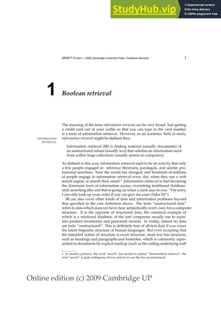
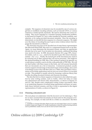
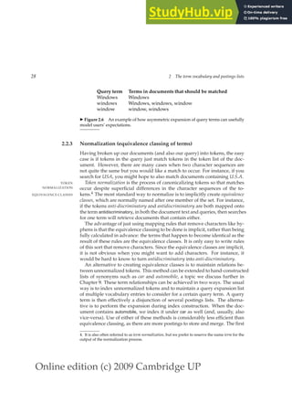
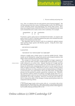
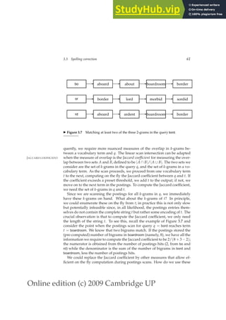
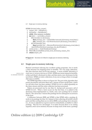
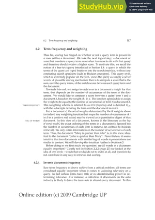
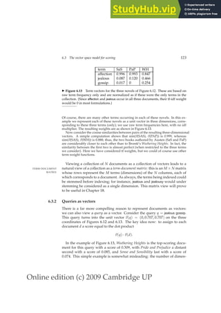
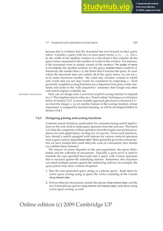
◮ Figure 1.2 Results from Shakespeare for the query Brutus AND Caesar AND NOT
Calpurnia.
we assume an average of 6 bytes per word including spaces and punctuation,
then this is a document collection about 6 GB in size. Typically, there might
be about M = 500,000 distinct terms in these documents. There is nothing
special about the numbers we have chosen, and they might vary by an order
of magnitude or more, but they give us some idea of the dimensions of the
kinds of problems we need to handle. We will discuss and model these size
assumptions in Section 5.1 (page 86).
Our goal is to develop a system to address the ad hoc retrieval task. This is
AD HOC RETRIEVAL
the most standard IR task. In it, a system aims to provide documents from
within the collection that are relevant to an arbitrary user information need,
communicated to the system by means of a one-off, user-initiated query. An
information need is the topic about which the user desires to know more, and
INFORMATION NEED
is differentiated from a query, which is what the user conveys to the com-
QUERY
puter in an attempt to communicate the information need. A document is
relevant if it is one that the user perceives as containing information of value
RELEVANCE
with respect to their personal information need. Our example above was
rather artificial in that the information need was defined in terms of par-
ticular words, whereas usually a user is interested in a topic like “pipeline
leaks” and would like to find relevant documents regardless of whether they
precisely use those words or express the concept with other words such as
pipeline rupture. To assess the effectiveness of an IR system (i.e., the quality of
EFFECTIVENESS
its search results), a user will usually want to know two key statistics about
the system’s returned results for a query:
Precision: What fraction of the returned results are relevant to the informa-
PRECISION
tion need?
Recall: What fraction of the relevant documents in the collection were re-
RECALL
turned by the system?](https://image.slidesharecdn.com/anintroductiontoinformationretrieval-230807170822-1d67eee0/85/An-Introduction-to-Information-Retrieval-pdf-30-320.jpg)

![Online edition (c) 2009 Cambridge UP
1.2 A first take at building an inverted index 9
search engine at query time, and it is a statistic later used in many ranked re-
trieval models. The postings are secondarily sorted by docID. This provides
the basis for efficient query processing. This inverted index structure is es-
sentially without rivals as the most efficient structure for supporting ad hoc
text search.
In the resulting index, we pay for storage of both the dictionary and the
postings lists. The latter are much larger, but the dictionary is commonly
kept in memory, while postings lists are normally kept on disk, so the size
of each is important, and in Chapter 5 we will examine how each can be
optimized for storage and access efficiency. What data structure should be
used for a postings list? A fixed length array would be wasteful as some
words occur in many documents, and others in very few. For an in-memory
postings list, two good alternatives are singly linked lists or variable length
arrays. Singly linked lists allow cheap insertion of documents into postings
lists (following updates, such as when recrawling the web for updated doc-
uments), and naturally extend to more advanced indexing strategies such as
skip lists (Section 2.3), which require additional pointers. Variable length ar-
rays win in space requirements by avoiding the overhead for pointers and in
time requirements because their use of contiguous memory increases speed
on modern processors with memory caches. Extra pointers can in practice be
encoded into the lists as offsets. If updates are relatively infrequent, variable
length arrays will be more compact and faster to traverse. We can also use a
hybrid scheme with a linked list of fixed length arrays for each term. When
postings lists are stored on disk, they are stored (perhaps compressed) as a
contiguous run of postings without explicit pointers (as in Figure 1.3), so as
to minimize the size of the postings list and the number of disk seeks to read
a postings list into memory.
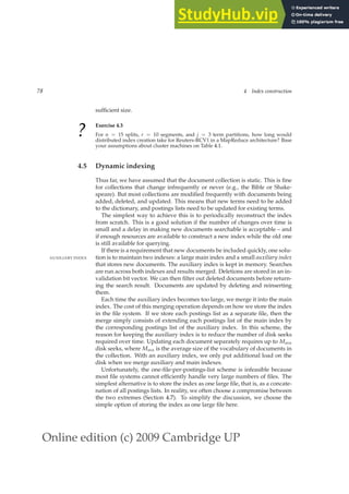
?
Exercise 1.1 [⋆]
Draw the inverted index that would be built for the following document collection.
(See Figure 1.3 for an example.)
Doc 1 new home sales top forecasts
Doc 2 home sales rise in july
Doc 3 increase in home sales in july
Doc 4 july new home sales rise
Exercise 1.2 [⋆]
Consider these documents:
Doc 1 breakthrough drug for schizophrenia
Doc 2 new schizophrenia drug
Doc 3 new approach for treatment of schizophrenia
Doc 4 new hopes for schizophrenia patients
a. Draw the term-document incidence matrix for this document collection.](https://image.slidesharecdn.com/anintroductiontoinformationretrieval-230807170822-1d67eee0/85/An-Introduction-to-Information-Retrieval-pdf-34-320.jpg)
![Online edition (c) 2009 Cambridge UP
10 1 Boolean retrieval
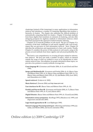
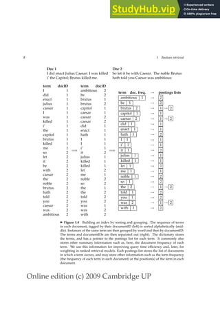
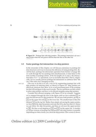
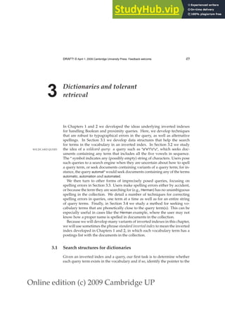
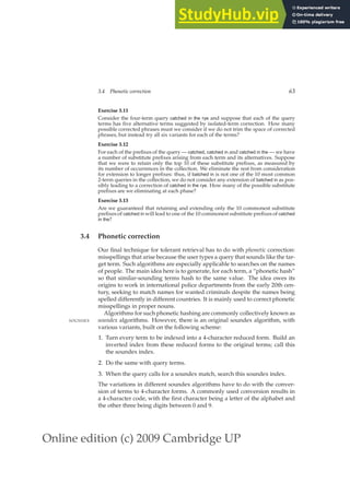
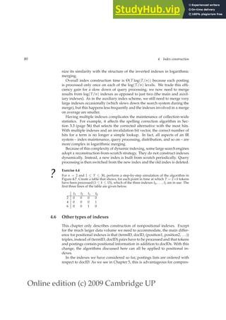
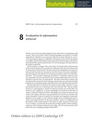
Brutus −→ 1 → 2 → 4 → 11 → 31 → 45 → 173 → 174
Calpurnia −→ 2 → 31 → 54 → 101
Intersection =⇒ 2 → 31
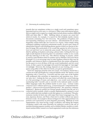
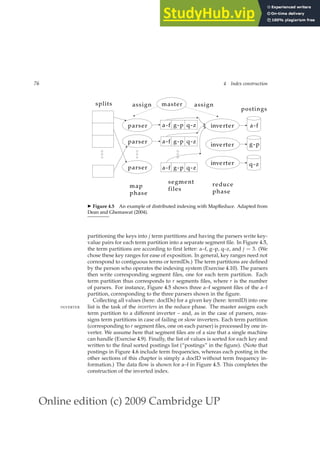
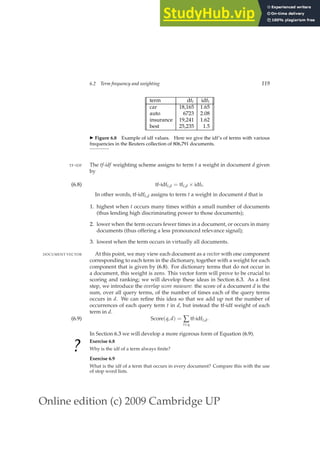
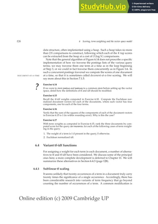
◮ Figure 1.5 Intersecting the postings lists for Brutus and Calpurnia from Figure 1.3.
b. Draw the inverted index representation for this collection, as in Figure 1.3 (page 7).
Exercise 1.3 [⋆]
For the document collection shown in Exercise 1.2, what are the returned results for
these queries:
a. schizophrenia AND drug
b. for AND NOT(drug OR approach)
1.3 Processing Boolean queries
How do we process a query using an inverted index and the basic Boolean
retrieval model? Consider processing the simple conjunctive query:
SIMPLE CONJUNCTIVE
QUERIES
(1.1) Brutus AND Calpurnia
over the inverted index partially shown in Figure 1.3 (page 7). We:
1. Locate Brutus in the Dictionary
2. Retrieve its postings
3. Locate Calpurnia in the Dictionary
4. Retrieve its postings
5. Intersect the two postings lists, as shown in Figure 1.5.
The intersection operation is the crucial one: we need to efficiently intersect
POSTINGS LIST
INTERSECTION postings lists so as to be able to quickly find documents that contain both
terms. (This operation is sometimes referred to as merging postings lists:
POSTINGS MERGE
this slightly counterintuitive name reflects using the term merge algorithm for
a general family of algorithms that combine multiple sorted lists by inter-
leaved advancing of pointers through each; here we are merging the lists
with a logical AND operation.)
There is a simple and effective method of intersecting postings lists using
the merge algorithm (see Figure 1.6): we maintain pointers into both lists](https://image.slidesharecdn.com/anintroductiontoinformationretrieval-230807170822-1d67eee0/85/An-Introduction-to-Information-Retrieval-pdf-35-320.jpg)

![Online edition (c) 2009 Cambridge UP
1.3 Processing Boolean queries 13
intersection can still be done by the algorithm in Figure 1.6, but when the
difference between the list lengths is very large, opportunities to use alter-
native techniques open up. The intersection can be calculated in place by
destructively modifying or marking invalid items in the intermediate results
list. Or the intersection can be done as a sequence of binary searches in the
long postings lists for each posting in the intermediate results list. Another
possibility is to store the long postings list as a hashtable, so that membership
of an intermediate result item can be calculated in constant rather than linear
or log time. However, such alternative techniques are difficult to combine
with postings list compression of the sort discussed in Chapter 5. Moreover,
standard postings list intersection operations remain necessary when both
terms of a query are very common.
?
Exercise 1.4 [⋆]
For the queries below, can we still run through the intersection in time O(x + y),
where x and y are the lengths of the postings lists for Brutus and Caesar? If not, what
can we achieve?
a. Brutus AND NOT Caesar
b. Brutus OR NOT Caesar
Exercise 1.5 [⋆]
Extend the postings merge algorithm to arbitrary Boolean query formulas. What is
its time complexity? For instance, consider:
c. (Brutus OR Caesar) AND NOT (Antony OR Cleopatra)
Can we always merge in linear time? Linear in what? Can we do better than this?
Exercise 1.6 [⋆⋆]
We can use distributive laws for AND and OR to rewrite queries.
a. Show how to rewrite the query in Exercise 1.5 into disjunctive normal form using
the distributive laws.
b. Would the resulting query be more or less efficiently evaluated than the original
form of this query?
c. Is this result true in general or does it depend on the words and the contents of
the document collection?
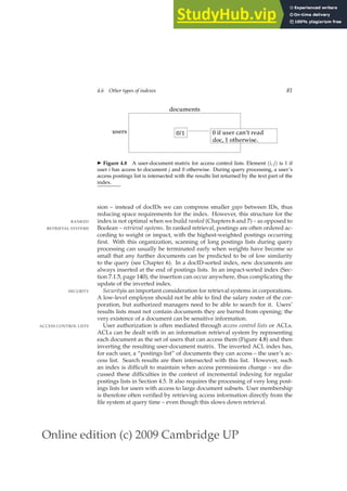
Exercise 1.7 [⋆]
Recommend a query processing order for
d. (tangerine OR trees) AND (marmalade OR skies) AND (kaleidoscope OR eyes)
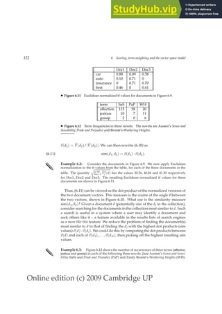
given the following postings list sizes:](https://image.slidesharecdn.com/anintroductiontoinformationretrieval-230807170822-1d67eee0/85/An-Introduction-to-Information-Retrieval-pdf-38-320.jpg)
![Online edition (c) 2009 Cambridge UP
14 1 Boolean retrieval
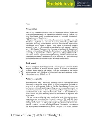
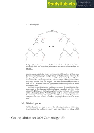
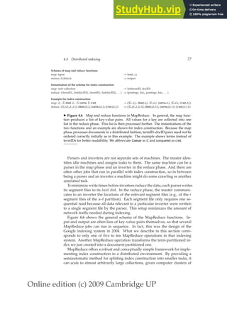
Term Postings size
eyes 213312
kaleidoscope 87009
marmalade 107913
skies 271658
tangerine 46653
trees 316812
Exercise 1.8 [⋆]
If the query is:
e. friends AND romans AND (NOT countrymen)
how could we use the frequency of countrymen in evaluating the best query evaluation
order? In particular, propose a way of handling negation in determining the order of
query processing.
Exercise 1.9 [⋆⋆]
For a conjunctive query, is processing postings lists in order of size guaranteed to be
optimal? Explain why it is, or give an example where it isn’t.
Exercise 1.10 [⋆⋆]
Write out a postings merge algorithm, in the style of Figure 1.6 (page 11), for an x OR y
query.
Exercise 1.11 [⋆⋆]
How should the Boolean query x AND NOT y be handled? Why is naive evaluation
of this query normally very expensive? Write out a postings merge algorithm that
evaluates this query efficiently.
1.4 The extended Boolean model versus ranked retrieval
The Boolean retrieval model contrasts with ranked retrieval models such as the
RANKED RETRIEVAL
MODEL vector space model (Section 6.3), in which users largely use free text queries,
FREE TEXT QUERIES
that is, just typing one or more words rather than using a precise language
with operators for building up query expressions, and the system decides
which documents best satisfy the query. Despite decades of academic re-
search on the advantages of ranked retrieval, systems implementing the Boo-
lean retrieval model were the main or only search option provided by large
commercial information providers for three decades until the early 1990s (ap-
proximately the date of arrival of the World Wide Web). However, these
systems did not have just the basic Boolean operations (AND, OR, and NOT)
which we have presented so far. A strict Boolean expression over terms with
an unordered results set is too limited for many of the information needs
that people have, and these systems implemented extended Boolean retrieval
models by incorporating additional operators such as term proximity oper-
ators. A proximity operator is a way of specifying that two terms in a query
PROXIMITY OPERATOR](https://image.slidesharecdn.com/anintroductiontoinformationretrieval-230807170822-1d67eee0/85/An-Introduction-to-Information-Retrieval-pdf-39-320.jpg)

![Online edition (c) 2009 Cambridge UP
16 1 Boolean retrieval
inverted index, comprising a dictionary and postings lists. We introduced
the Boolean retrieval model, and examined how to do efficient retrieval via
linear time merges and simple query optimization. In Chapters 2–7 we will
consider in detail richer query models and the sort of augmented index struc-
tures that are needed to handle them efficiently. Here we just mention a few
of the main additional things we would like to be able to do:
1. We would like to better determine the set of terms in the dictionary and
to provide retrieval that is tolerant to spelling mistakes and inconsistent
choice of words.
2. It is often useful to search for compounds or phrases that denote a concept
such as “operating system”. As the Westlaw examples show, we might also
wish to do proximity queries such as Gates NEAR Microsoft. To answer
such queries, the index has to be augmented to capture the proximities of
terms in documents.
3. A Boolean model only records term presence or absence, but often we
would like to accumulate evidence, giving more weight to documents that
have a term several times as opposed to ones that contain it only once. To
be able to do this we need term frequency information (the number of times
TERM FREQUENCY
a term occurs in a document) in postings lists.
4. Boolean queries just retrieve a set of matching documents, but commonly
we wish to have an effective method to order (or “rank”) the returned
results. This requires having a mechanism for determining a document
score which encapsulates how good a match a document is for a query.
With these additional ideas, we will have seen most of the basic technol-
ogy that supports ad hoc searching over unstructured information. Ad hoc
searching over documents has recently conquered the world, powering not
only web search engines but the kind of unstructured search that lies behind
the large eCommerce websites. Although the main web search engines differ
by emphasizing free text querying, most of the basic issues and technologies
of indexing and querying remain the same, as we will see in later chapters.
Moreover, over time, web search engines have added at least partial imple-
mentations of some of the most popular operators from extended Boolean
models: phrase search is especially popular and most have a very partial
implementation of Boolean operators. Nevertheless, while these options are
liked by expert searchers, they are little used by most people and are not the
main focus in work on trying to improve web search engine performance.
?
Exercise 1.12 [⋆]
Write a query using Westlaw syntax which would find any of the words professor,
teacher, or lecturer in the same sentence as a form of the verb explain.](https://image.slidesharecdn.com/anintroductiontoinformationretrieval-230807170822-1d67eee0/85/An-Introduction-to-Information-Retrieval-pdf-41-320.jpg)
![Online edition (c) 2009 Cambridge UP
1.5 References and further reading 17
Exercise 1.13 [⋆]
Try using the Boolean search features on a couple of major web search engines. For
instance, choose a word, such as burglar, and submit the queries (i) burglar, (ii) burglar
AND burglar, and (iii) burglar OR burglar. Look at the estimated number of results and
top hits. Do they make sense in terms of Boolean logic? Often they haven’t for major
search engines. Can you make sense of what is going on? What about if you try
different words? For example, query for (i) knight, (ii) conquer, and then (iii) knight OR
conquer. What bound should the number of results from the first two queries place
on the third query? Is this bound observed?
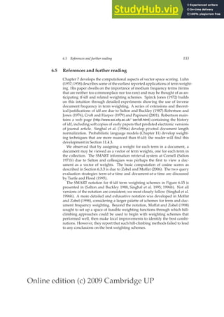
1.5 References and further reading
The practical pursuit of computerized information retrieval began in the late
1940s (Cleverdon 1991, Liddy 2005). A great increase in the production of
scientific literature, much in the form of less formal technical reports rather
than traditional journal articles, coupled with the availability of computers,
led to interest in automatic document retrieval. However, in those days, doc-
ument retrieval was always based on author, title, and keywords; full-text
search came much later.
The article of Bush (1945) provided lasting inspiration for the new field:
“Consider a future device for individual use, which is a sort of mech-
anized private file and library. It needs a name, and, to coin one at
random, ‘memex’ will do. A memex is a device in which an individual
stores all his books, records, and communications, and which is mech-
anized so that it may be consulted with exceeding speed and flexibility.
It is an enlarged intimate supplement to his memory.”
The term Information Retrieval was coined by Calvin Mooers in 1948/1950
(Mooers 1950).
In 1958, much newspaper attention was paid to demonstrations at a con-
ference (see Taube and Wooster 1958) of IBM “auto-indexing” machines, based
primarily on the work of H. P. Luhn. Commercial interest quickly gravitated
towards Boolean retrieval systems, but the early years saw a heady debate
over various disparate technologies for retrieval systems. For example Moo-
ers (1961) dissented:
“It is a common fallacy, underwritten at this date by the investment of
several million dollars in a variety of retrieval hardware, that the al-
gebra of George Boole (1847) is the appropriate formalism for retrieval
system design. This view is as widely and uncritically accepted as it is
wrong.”
The observation of AND vs. OR giving you opposite extremes in a precision/
recall tradeoff, but not the middle ground comes from (Lee and Fox 1988).](https://image.slidesharecdn.com/anintroductiontoinformationretrieval-230807170822-1d67eee0/85/An-Introduction-to-Information-Retrieval-pdf-42-320.jpg)


![Online edition (c) 2009 Cambridge UP
2.2 Determining the vocabulary of terms 35
? Exercise 2.1 [⋆]
Are the following statements true or false?
a. In a Boolean retrieval system, stemming never lowers precision.
b. In a Boolean retrieval system, stemming never lowers recall.
c. Stemming increases the size of the vocabulary.
d. Stemming should be invoked at indexing time but not while processing a query.
Exercise 2.2 [⋆]
Suggest what normalized form should be used for these words (including the word
itself as a possibility):
a. ’Cos
b. Shi’ite
c. cont’d
d. Hawai’i
e. O’Rourke
Exercise 2.3 [⋆]
The following pairs of words are stemmed to the same form by the Porter stemmer.
Which pairs would you argue shouldn’t be conflated. Give your reasoning.
a. abandon/abandonment
b. absorbency/absorbent
c. marketing/markets
d. university/universe
e. volume/volumes
Exercise 2.4 [⋆]
For the Porter stemmer rule group shown in (2.1):
a. What is the purpose of including an identity rule such as SS → SS?
b. Applying just this rule group, what will the following words be stemmed to?
circus canaries boss
c. What rule should be added to correctly stem pony?
d. The stemming for ponies and pony might seem strange. Does it have a deleterious
effect on retrieval? Why or why not?](https://image.slidesharecdn.com/anintroductiontoinformationretrieval-230807170822-1d67eee0/85/An-Introduction-to-Information-Retrieval-pdf-60-320.jpg)
![Online edition (c) 2009 Cambridge UP
38 2 The term vocabulary and postings lists
ory then the equation changes again. We discuss the impact of hardware
parameters on index construction time in Section 4.1 (page 68) and the im-
pact of index size on system speed in Chapter 5.
?
Exercise 2.5 [⋆]
Why are skip pointers not useful for queries of the form x OR y?
Exercise 2.6 [⋆]
We have a two-word query. For one term the postings list consists of the following 16
entries:
[4,6,10,12,14,16,18,20,22,32,47,81,120,122,157,180]
and for the other it is the one entry postings list:
[47].
Work out how many comparisons would be done to intersect the two postings lists
with the following two strategies. Briefly justify your answers:
a. Using standard postings lists
b. Using postings lists stored with skip pointers, with a skip length of
√
P, as sug-
gested in Section 2.3.
Exercise 2.7 [⋆]
Consider a postings intersection between this postings list, with skip pointers:
3 5 9 15 24 39 60 68 75 81 84 89 92 96 97 100 115
and the following intermediate result postings list (which hence has no skip pointers):
3 5 89 95 97 99 100 101
Trace through the postings intersection algorithm in Figure 2.10 (page 37).
a. How often is a skip pointer followed (i.e., p1 is advanced to skip(p1))?
b. How many postings comparisons will be made by this algorithm while intersect-
ing the two lists?
c. How many postings comparisons would be made if the postings lists are inter-
sected without the use of skip pointers?](https://image.slidesharecdn.com/anintroductiontoinformationretrieval-230807170822-1d67eee0/85/An-Introduction-to-Information-Retrieval-pdf-63-320.jpg)


![Online edition (c) 2009 Cambridge UP
42 2 The term vocabulary and postings lists
POSITIONALINTERSECT(p1, p2, k)
1 answer ← h i
2 while p1 6= NIL and p2 6= NIL
3 do if docID(p1) = docID(p2)
4 then l ← h i
5 pp1 ← positions(p1)
6 pp2 ← positions(p2)
7 while pp1 6= NIL
8 do while pp2 6= NIL
9 do if |pos(pp1) − pos(pp2)| ≤ k
10 then ADD(l, pos(pp2))
11 else if pos(pp2) pos(pp1)
12 then break
13 pp2 ← next(pp2)
14 while l 6= h i and |l[0] − pos(pp1)| k
15 do DELETE(l[0])
16 for each ps ∈ l
17 do ADD(answer, hdocID(p1), pos(pp1), psi)
18 pp1 ← next(pp1)
19 p1 ← next(p1)
20 p2 ← next(p2)
21 else if docID(p1) docID(p2)
22 then p1 ← next(p1)
23 else p2 ← next(p2)
24 return answer
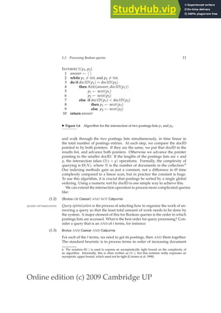
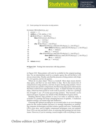
◮ Figure 2.12 An algorithm for proximity intersection of postings lists p1 and p2.
The algorithm finds places where the two terms appear within k words of each other
and returns a list of triples giving docID and the term position in p1 and p2.
The same general method is applied for within k word proximity searches,
of the sort we saw in Example 1.1 (page 15):
employment /3 place
Here, /k means “within k words of (on either side)”. Clearly, positional in-
dexes can be used for such queries; biword indexes cannot. We show in
Figure 2.12 an algorithm for satisfying within k word proximity searches; it
is further discussed in Exercise 2.12.
Positional index size. Adopting a positional index expands required post-
ings storage significantly, even if we compress position values/offsets as we](https://image.slidesharecdn.com/anintroductiontoinformationretrieval-230807170822-1d67eee0/85/An-Introduction-to-Information-Retrieval-pdf-67-320.jpg)
![Online edition (c) 2009 Cambridge UP
44 2 The term vocabulary and postings lists
Williams et al. (2004) evaluate an even more sophisticated scheme which
employs indexes of both these sorts and additionally a partial next word
index as a halfway house between the first two strategies. For each term, a
next word index records terms that follow it in a document. They conclude
NEXT WORD INDEX
that such a strategy allows a typical mixture of web phrase queries to be
completed in one quarter of the time taken by use of a positional index alone,
while taking up 26% more space than use of a positional index alone.
? Exercise 2.8 [⋆]
Assume a biword index. Give an example of a document which will be returned
for a query of New York University but is actually a false positive which should not be
returned.
Exercise 2.9 [⋆]
Shown below is a portion of a positional index in the format: term: doc1: hposition1,
position2, . . . i; doc2: hposition1, position2, . . . i; etc.
angels: 2: h36,174,252,651i; 4: h12,22,102,432i; 7: h17i;
fools: 2: h1,17,74,222i; 4: h8,78,108,458i; 7: h3,13,23,193i;
fear: 2: h87,704,722,901i; 4: h13,43,113,433i; 7: h18,328,528i;
in: 2: h3,37,76,444,851i; 4: h10,20,110,470,500i; 7: h5,15,25,195i;
rush: 2: h2,66,194,321,702i; 4: h9,69,149,429,569i; 7: h4,14,404i;
to: 2: h47,86,234,999i; 4: h14,24,774,944i; 7: h199,319,599,709i;
tread: 2: h57,94,333i; 4: h15,35,155i; 7: h20,320i;
where: 2: h67,124,393,1001i; 4: h11,41,101,421,431i; 7: h16,36,736i;
Which document(s) if any match each of the following queries, where each expression
within quotes is a phrase query?
a. “fools rush in”
b. “fools rush in” AND “angels fear to tread”
Exercise 2.10 [⋆]
Consider the following fragment of a positional index with the format:
word: document: hposition, position, . . .i; document: hposition, . . .i
. . .
Gates: 1: h3i; 2: h6i; 3: h2,17i; 4: h1i;
IBM: 4: h3i; 7: h14i;
Microsoft: 1: h1i; 2: h1,21i; 3: h3i; 5: h16,22,51i;
The /k operator, word1 /k word2 finds occurrences of word1 within k words of word2 (on
either side), where k is a positive integer argument. Thus k = 1 demands that word1
be adjacent to word2.
a. Describe the set of documents that satisfy the query Gates /2 Microsoft.
b. Describe each set of values for k for which the query Gates /k Microsoft returns a
different set of documents as the answer.](https://image.slidesharecdn.com/anintroductiontoinformationretrieval-230807170822-1d67eee0/85/An-Introduction-to-Information-Retrieval-pdf-69-320.jpg)
![Online edition (c) 2009 Cambridge UP
2.5 References and further reading 45
Exercise 2.11 [⋆⋆]
Consider the general procedure for merging two positional postings lists for a given
document, to determine the document positions where a document satisfies a /k
clause (in general there can be multiple positions at which each term occurs in a sin-
gle document). We begin with a pointer to the position of occurrence of each term
and move each pointer along the list of occurrences in the document, checking as we
do so whether we have a hit for /k. Each move of either pointer counts as a step. Let
L denote the total number of occurrences of the two terms in the document. What is
the big-O complexity of the merge procedure, if we wish to have postings including
positions in the result?
Exercise 2.12 [⋆⋆]
Consider the adaptation of the basic algorithm for intersection of two postings lists
(Figure 1.6, page 11) to the one in Figure 2.12 (page 42), which handles proximity
queries. A naive algorithm for this operation could be O(PLmax
2), where P is the
sum of the lengths of the postings lists (i.e., the sum of document frequencies) and
Lmax is the maximum length of a document (in tokens).
a. Go through this algorithm carefully and explain how it works.
b. What is the complexity of this algorithm? Justify your answer carefully.
c. For certain queries and data distributions, would another algorithm be more effi-
cient? What complexity does it have?
Exercise 2.13 [⋆⋆]
Suppose we wish to use a postings intersection procedure to determine simply the
list of documents that satisfy a /k clause, rather than returning the list of positions,
as in Figure 2.12 (page 42). For simplicity, assume k ≥ 2. Let L denote the total
number of occurrences of the two terms in the document collection (i.e., the sum of
their collection frequencies). Which of the following is true? Justify your answer.
a. The merge can be accomplished in a number of steps linear in L and independent
of k, and we can ensure that each pointer moves only to the right.
b. The merge can be accomplished in a number of steps linear in L and independent
of k, but a pointer may be forced to move non-monotonically (i.e., to sometimes
back up)
c. The merge can require kL steps in some cases.
Exercise 2.14 [⋆⋆]
How could an IR system combine use of a positional index and use of stop words?
What is the potential problem, and how could it be handled?
2.5 References and further reading
Exhaustive discussion of the character-level processing of East Asian lan-
EAST ASIAN
LANGUAGES guages can be found in Lunde (1998). Character bigram indexes are perhaps
the most standard approach to indexing Chinese, although some systems use
word segmentation. Due to differences in the language and writing system,
word segmentation is most usual for Japanese (Luk and Kwok 2002, Kishida](https://image.slidesharecdn.com/anintroductiontoinformationretrieval-230807170822-1d67eee0/85/An-Introduction-to-Information-Retrieval-pdf-70-320.jpg)


![Online edition (c) 2009 Cambridge UP
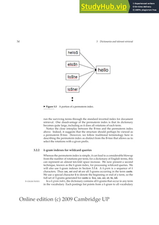
50 3 Dictionaries and tolerant retrieval
corresponding postings. This vocabulary lookup operation uses a classical
data structure called the dictionary and has two broad classes of solutions:
hashing, and search trees. In the literature of data structures, the entries in
the vocabulary (in our case, terms) are often referred to as keys. The choice
of solution (hashing, or search trees) is governed by a number of questions:
(1) How many keys are we likely to have? (2) Is the number likely to remain
static, or change a lot – and in the case of changes, are we likely to only have
new keys inserted, or to also have some keys in the dictionary be deleted? (3)
What are the relative frequencies with which various keys will be accessed?
Hashing has been used for dictionary lookup in some search engines. Each
vocabulary term (key) is hashed into an integer over a large enough space
that hash collisions are unlikely; collisions if any are resolved by auxiliary
structures that can demand care to maintain.1 At query time, we hash each
query term separately and following a pointer to the corresponding post-
ings, taking into account any logic for resolving hash collisions. There is no
easy way to find minor variants of a query term (such as the accented and
non-accented versions of a word like resume), since these could be hashed to
very different integers. In particular, we cannot seek (for instance) all terms
beginning with the prefix automat, an operation that we will require below
in Section 3.2. Finally, in a setting (such as the Web) where the size of the
vocabulary keeps growing, a hash function designed for current needs may
not suffice in a few years’ time.
Search trees overcome many of these issues – for instance, they permit us
to enumerate all vocabulary terms beginning with automat. The best-known
search tree is the binary tree, in which each internal node has two children.
BINARY TREE
The search for a term begins at the root of the tree. Each internal node (in-
cluding the root) represents a binary test, based on whose outcome the search
proceeds to one of the two sub-trees below that node. Figure 3.1 gives an ex-
ample of a binary search tree used for a dictionary. Efficient search (with a
number of comparisons that is O(log M)) hinges on the tree being balanced:
the numbers of terms under the two sub-trees of any node are either equal
or differ by one. The principal issue here is that of rebalancing: as terms are
inserted into or deleted from the binary search tree, it needs to be rebalanced
so that the balance property is maintained.
To mitigate rebalancing, one approach is to allow the number of sub-trees
under an internal node to vary in a fixed interval. A search tree commonly
used for a dictionary is the B-tree – a search tree in which every internal node
B-TREE
has a number of children in the interval [a, b], where a and b are appropriate
positive integers; Figure 3.2 shows an example with a = 2 and b = 4. Each
branch under an internal node again represents a test for a range of char-
1. So-called perfect hash functions are designed to preclude collisions, but are rather more com-
plicated both to implement and to compute.](https://image.slidesharecdn.com/anintroductiontoinformationretrieval-230807170822-1d67eee0/85/An-Introduction-to-Information-Retrieval-pdf-75-320.jpg)


![Online edition (c) 2009 Cambridge UP
58 3 Dictionaries and tolerant retrieval
have a multiple-term query. The carot example demonstrates this type of cor-
rection. Such isolated-term correction would fail to detect, for instance, that
the query flew form Heathrow contains a mis-spelling of the term from – because
each term in the query is correctly spelled in isolation.
We begin by examining two techniques for addressing isolated-term cor-
rection: edit distance, and k-gram overlap. We then proceed to context-
sensitive correction.
3.3.3 Edit distance
Given two character strings s1 and s2, the edit distance between them is the
EDIT DISTANCE
minimum number of edit operations required to transform s1 into s2. Most
commonly, the edit operations allowed for this purpose are: (i) insert a char-
acter into a string; (ii) delete a character from a string and (iii) replace a char-
acter of a string by another character; for these operations, edit distance is
sometimes known as Levenshtein distance. For example, the edit distance be-
LEVENSHTEIN
DISTANCE tween cat and dog is 3. In fact, the notion of edit distance can be generalized
to allowing different weights for different kinds of edit operations, for in-
stance a higher weight may be placed on replacing the character s by the
character p, than on replacing it by the character a (the latter being closer to s
on the keyboard). Setting weights in this way depending on the likelihood of
letters substituting for each other is very effective in practice (see Section 3.4
for the separate issue of phonetic similarity). However, the remainder of our
treatment here will focus on the case in which all edit operations have the
same weight.
It is well-known how to compute the (weighted) edit distance between
two strings in time O(|s1| × |s2|), where |si| denotes the length of a string si.
The idea is to use the dynamic programming algorithm in Figure 3.5, where
the characters in s1 and s2 are given in array form. The algorithm fills the
(integer) entries in a matrix m whose two dimensions equal the lengths of
the two strings whose edit distances is being computed; the (i, j) entry of the
matrix will hold (after the algorithm is executed) the edit distance between
the strings consisting of the first i characters of s1 and the first j characters
of s2. The central dynamic programming step is depicted in Lines 8-10 of
Figure 3.5, where the three quantities whose minimum is taken correspond
to substituting a character in s1, inserting a character in s1 and inserting a
character in s2.
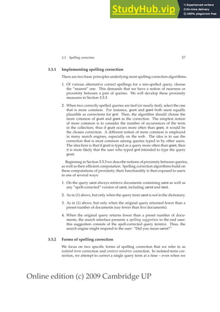
Figure 3.6 shows an example Levenshtein distance computation of Fig-
ure 3.5. The typical cell [i, j] has four entries formatted as a 2 × 2 cell. The
lower right entry in each cell is the min of the other three, corresponding to
the main dynamic programming step in Figure 3.5. The other three entries
are the three entries m[i − 1, j − 1] + 0 or 1 depending on whether s1[i] =](https://image.slidesharecdn.com/anintroductiontoinformationretrieval-230807170822-1d67eee0/85/An-Introduction-to-Information-Retrieval-pdf-83-320.jpg)
![Online edition (c) 2009 Cambridge UP
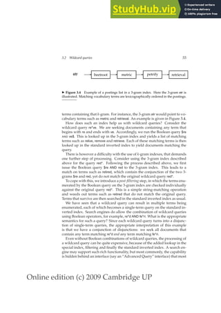
3.3 Spelling correction 59
EDITDISTANCE(s1, s2)
1 int m[i, j] = 0
2 for i ← 1 to |s1|
3 do m[i, 0] = i
4 for j ← 1 to |s2|
5 do m[0, j] = j
6 for i ← 1 to |s1|
7 do for j ← 1 to |s2|
8 do m[i, j] = min{m[i − 1, j − 1] + if (s1[i] = s2[j]) then 0 else 1fi,
9 m[i − 1, j] + 1,
10 m[i, j − 1] + 1}
11 return m[|s1|, |s2|]
◮ Figure 3.5 Dynamic programming algorithm for computing the edit distance be-
tween strings s1 and s2.
f a s t
0 1 1 2 2 3 3 4 4
c
1
1
1 2
2 1
2 3
2 2
3 4
3 3
4 5
4 4
a
2
2
2 2
3 2
1 3
3 1
3 4
2 2
4 5
3 3
t
3
3
3 3
4 3
3 2
4 2
2 3
3 2
2 4
3 2
s
4
4
4 4
5 4
4 3
5 3
2 3
4 2
3 3
3 3
◮ Figure 3.6 Example Levenshtein distance computation. The 2 × 2 cell in the [i, j]
entry of the table shows the three numbers whose minimum yields the fourth. The
cells in italics determine the edit distance in this example.
s2[j], m[i − 1, j] + 1 and m[i, j − 1] + 1. The cells with numbers in italics depict
the path by which we determine the Levenshtein distance.
The spelling correction problem however demands more than computing
edit distance: given a set S of strings (corresponding to terms in the vocab-
ulary) and a query string q, we seek the string(s) in V of least edit distance
from q. We may view this as a decoding problem, in which the codewords
(the strings in V) are prescribed in advance. The obvious way of doing this
is to compute the edit distance from q to each string in V, before selecting the](https://image.slidesharecdn.com/anintroductiontoinformationretrieval-230807170822-1d67eee0/85/An-Introduction-to-Information-Retrieval-pdf-84-320.jpg)


![Online edition (c) 2009 Cambridge UP
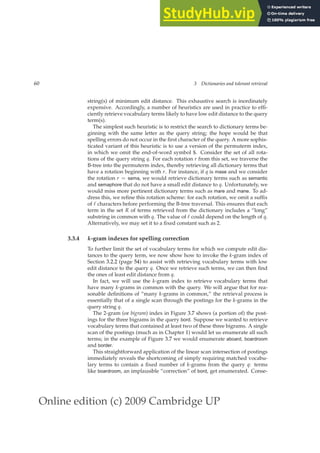
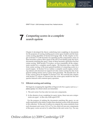
70 4 Index construction
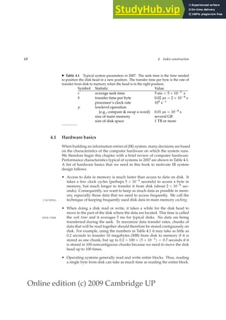
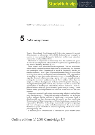
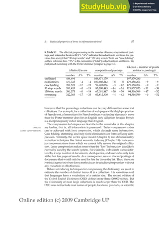
◮ Table 4.2 Collection statistics for Reuters-RCV1. Values are rounded for the com-
putations in this book. The unrounded values are: 806,791 documents, 222 tokens
per document, 391,523 (distinct) terms, 6.04 bytes per token with spaces and punc-
tuation, 4.5 bytes per token without spaces and punctuation, 7.5 bytes per term, and
96,969,056 tokens. The numbers in this table correspond to the third line (“case fold-
ing”) in Table 5.1 (page 87).
Symbol Statistic Value
N documents 800,000
Lave avg. # tokens per document 200
M terms 400,000
avg. # bytes per token (incl. spaces/punct.) 6
avg. # bytes per token (without spaces/punct.) 4.5
avg. # bytes per term 7.5
T tokens 100,000,000
REUTERS
Extreme conditions create rare Antarctic clouds
You are here: Home News Science Article
Go to a Section: U.S. International Business Markets Politics Entertainment Technology
Tue Aug 1, 2006 3:20am ET
Email This Article | Print This Article | Reprints
SYDNEY (Reuters) - Rare, mother-of-pearl colored clouds
caused by extreme weather conditions above Antarctica are a
possible indication of global warming, Australian scientists said on
Tuesday.
Known as nacreous clouds, the spectacular formations showing delicate
wisps of colors were photographed in the sky over an Australian
meteorological base at Mawson Station on July 25.
Sports Oddly Enough
[-] Text [+]
◮ Figure 4.1 Document from the Reuters newswire.
Reuters-RCV1 has 100 million tokens. Collecting all termID–docID pairs of
the collection using 4 bytes each for termID and docID therefore requires 0.8
GB of storage. Typical collections today are often one or two orders of mag-
nitude larger than Reuters-RCV1. You can easily see how such collections
overwhelm even large computers if we try to sort their termID–docID pairs
in memory. If the size of the intermediate files during index construction is
within a small factor of available memory, then the compression techniques
introduced in Chapter 5 can help; however, the postings file of many large
collections cannot fit into memory even after compression.
With main memory insufficient, we need to use an external sorting algo-
EXTERNAL SORTING
ALGORITHM rithm, that is, one that uses disk. For acceptable speed, the central require-](https://image.slidesharecdn.com/anintroductiontoinformationretrieval-230807170822-1d67eee0/85/An-Introduction-to-Information-Retrieval-pdf-95-320.jpg)
![Online edition (c) 2009 Cambridge UP
72 4 Index construction
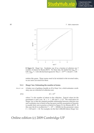
brutus d1,d3
caesar d1,d2,d4
noble d5
with d1,d2,d3,d5
brutus d6,d7
caesar d8,d9
julius d10
killed d8
postings lists
to be merged
brutus d1,d3,d6,d7
caesar d1,d2,d4,d8,d9
julius d10
killed d8
noble d5
with d1,d2,d3,d5
merged
postings lists
disk
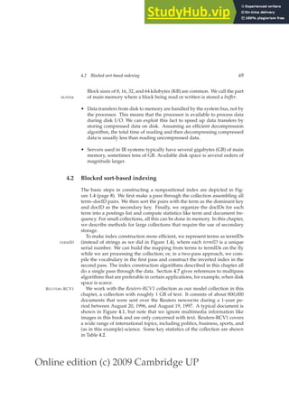
◮ Figure 4.3 Merging in blocked sort-based indexing. Two blocks (“postings lists to
be merged”) are loaded from disk into memory, merged in memory (“merged post-
ings lists”) and written back to disk. We show terms instead of termIDs for better
readability.
the actual indexing time is usually dominated by the time it takes to parse the
documents (PARSENEXTBLOCK) and to do the final merge (MERGEBLOCKS).
Exercise 4.6 asks you to compute the total index construction time for RCV1
that includes these steps as well as inverting the blocks and writing them to
disk.
Notice that Reuters-RCV1 is not particularly large in an age when one or
more GB of memory are standard on personal computers. With appropriate
compression (Chapter 5), we could have created an inverted index for RCV1
in memory on a not overly beefy server. The techniques we have described
are needed, however, for collections that are several orders of magnitude
larger.
? Exercise 4.1
If we need T log2 T comparisons (where T is the number of termID–docID pairs) and
two disk seeks for each comparison, how much time would index construction for
Reuters-RCV1 take if we used disk instead of memory for storage and an unopti-
mized sorting algorithm (i.e., not an external sorting algorithm)? Use the system
parameters in Table 4.1.
Exercise 4.2 [⋆]
How would you create the dictionary in blocked sort-based indexing on the fly to
avoid an extra pass through the data?](https://image.slidesharecdn.com/anintroductiontoinformationretrieval-230807170822-1d67eee0/85/An-Introduction-to-Information-Retrieval-pdf-97-320.jpg)


![Online edition (c) 2009 Cambridge UP
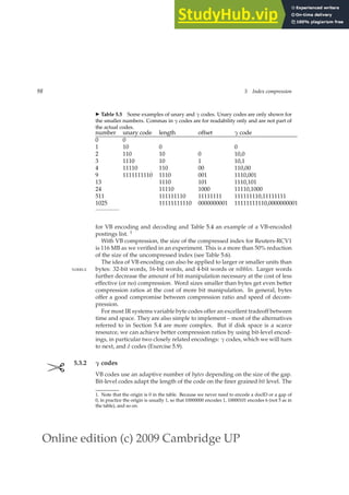
90 5 Index compression
0 1 2 3 4 5 6
0
1
2
3
4
5
6
7
log10 rank
7
log10
cf
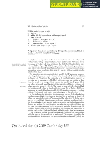
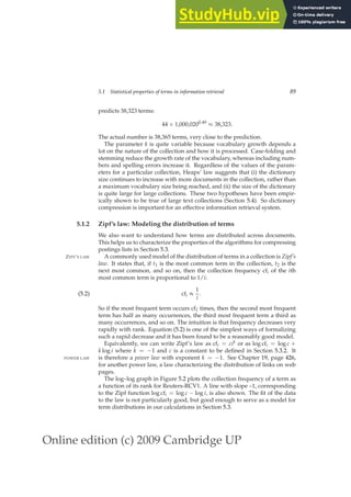
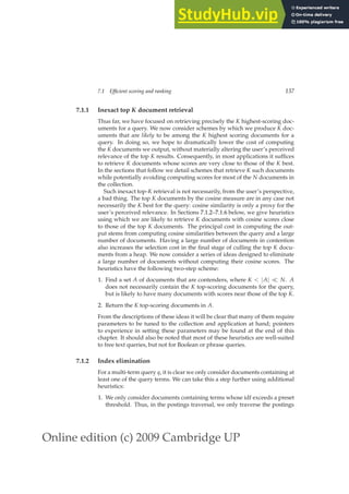
◮ Figure 5.2 Zipf’s law for Reuters-RCV1. Frequency is plotted as a function of
frequency rank for the terms in the collection. The line is the distribution predicted
by Zipf’s law (weighted least-squares fit; intercept is 6.95).
?
Exercise 5.1 [⋆]
Assuming one machine word per posting, what is the size of the uncompressed (non-
positional) index for different tokenizations based on Table 5.1? How do these num-
bers compare with Table 5.6?
5.2 Dictionary compression
This section presents a series of dictionary data structures that achieve in-
creasingly higher compression ratios. The dictionary is small compared with
the postings file as suggested by Table 5.1. So why compress it if it is respon-
sible for only a small percentage of the overall space requirements of the IR
system?
One of the primary factors in determining the response time of an IR sys-
tem is the number of disk seeks necessary to process a query. If parts of the
dictionary are on disk, then many more disk seeks are necessary in query
evaluation. Thus, the main goal of compressing the dictionary is to fit it in
main memory, or at least a large portion of it, to support high query through-](https://image.slidesharecdn.com/anintroductiontoinformationretrieval-230807170822-1d67eee0/85/An-Introduction-to-Information-Retrieval-pdf-115-320.jpg)


![Online edition (c) 2009 Cambridge UP
5.3 Postings file compression 95
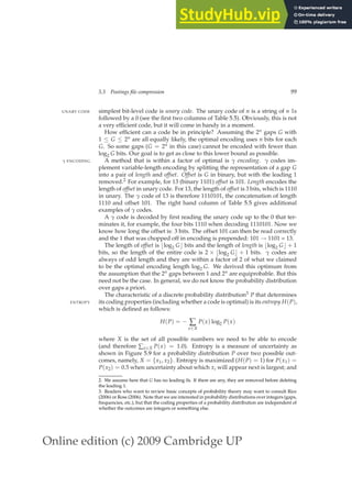
◮ Table 5.2 Dictionary compression for Reuters-RCV1.
data structure size in MB
dictionary, fixed-width 11.2
dictionary, term pointers into string 7.6
∼, with blocking, k = 4 7.1
∼, with blocking front coding 5.9
is identified for a subsequence of the term list and then referred to with a
special character. In the case of Reuters, front coding saves another 1.2 MB,
as we found in an experiment.
Other schemes with even greater compression rely on minimal perfect
hashing, that is, a hash function that maps M terms onto [1, . . . , M] without
collisions. However, we cannot adapt perfect hashes incrementally because
each new term causes a collision and therefore requires the creation of a new
perfect hash function. Therefore, they cannot be used in a dynamic environ-
ment.
Even with the best compression scheme, it may not be feasible to store
the entire dictionary in main memory for very large text collections and for
hardware with limited memory. If we have to partition the dictionary onto
pages that are stored on disk, then we can index the first term of each page
using a B-tree. For processing most queries, the search system has to go to
disk anyway to fetch the postings. One additional seek for retrieving the
term’s dictionary page from disk is a significant, but tolerable increase in the
time it takes to process a query.
Table 5.2 summarizes the compression achieved by the four dictionary
data structures.
?
Exercise 5.2
Estimate the space usage of the Reuters-RCV1 dictionary with blocks of size k = 8
and k = 16 in blocked dictionary storage.
Exercise 5.3
Estimate the time needed for term lookup in the compressed dictionary of Reuters-
RCV1 with block sizes of k = 4 (Figure 5.6, b), k = 8, and k = 16. What is the
slowdown compared with k = 1 (Figure 5.6, a)?
5.3 Postings file compression
Recall from Table 4.2 (page 70) that Reuters-RCV1 has 800,000 documents,
200 tokens per document, six characters per token, and 100,000,000 post-
ings where we define a posting in this chapter as a docID in a postings
list, that is, excluding frequency and position information. These numbers](https://image.slidesharecdn.com/anintroductiontoinformationretrieval-230807170822-1d67eee0/85/An-Introduction-to-Information-Retrieval-pdf-120-320.jpg)

![Online edition (c) 2009 Cambridge UP
5.3 Postings file compression 97
VBENCODENUMBER(n)
1 bytes ← hi
2 while true
3 do PREPEND(bytes, n mod 128)
4 if n 128
5 then BREAK
6 n ← n div 128
7 bytes[LENGTH(bytes)] += 128
8 return bytes
VBENCODE(numbers)
1 bytestream ← hi
2 for each n ∈ numbers
3 do bytes ← VBENCODENUMBER(n)
4 bytestream ← EXTEND(bytestream, bytes)
5 return bytestream
VBDECODE(bytestream)
1 numbers ← hi
2 n ← 0
3 for i ← 1 to LENGTH(bytestream)
4 do if bytestream[i] 128
5 then n ← 128 × n + bytestream[i]
6 else n ← 128 × n + (bytestream[i] − 128)
7 APPEND(numbers, n)
8 n ← 0
9 return numbers
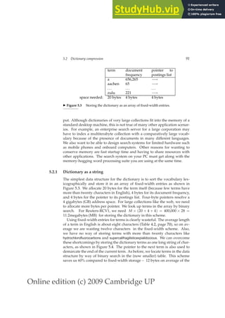
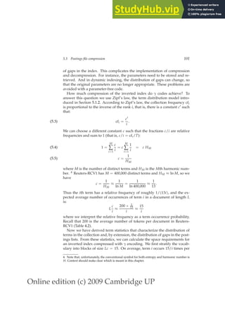
◮ Figure 5.8 VB encoding and decoding. The functions div and mod compute
integer division and remainder after integer division, respectively. PREPEND adds an
element to the beginning of a list, for example, PREPEND(h1,2i, 3) = h3, 1, 2i. EXTEND
extends a list, for example, EXTEND(h1,2i, h3, 4i) = h1, 2, 3, 4i.
◮ Table 5.4 VB encoding. Gaps are encoded using an integral number of bytes.
The first bit, the continuation bit, of each byte indicates whether the code ends with
this byte (1) or not (0).
docIDs 824 829 215406
gaps 5 214577
VB code 00000110 10111000 10000101 00001101 00001100 10110001](https://image.slidesharecdn.com/anintroductiontoinformationretrieval-230807170822-1d67eee0/85/An-Introduction-to-Information-Retrieval-pdf-122-320.jpg)


![Online edition (c) 2009 Cambridge UP
104 5 Index compression
somewhere in the middle of a machine word. As a result, query processing is
more expensive for γ codes than for variable byte codes. Whether we choose
variable byte or γ encoding depends on the characteristics of an application,
for example, on the relative weights we give to conserving disk space versus
maximizing query response time.
The compression ratio for the index in Table 5.6 is about 25%: 400 MB (un-
compressed, each posting stored as a 32-bit word) versus 101 MB (γ) and 116
MB (VB). This shows that both γ and VB codes meet the objectives we stated
in the beginning of the chapter. Index compression substantially improves
time and space efficiency of indexes by reducing the amount of disk space
needed, increasing the amount of information that can be kept in the cache,
and speeding up data transfers from disk to memory.
?
Exercise 5.4 [⋆]
Compute variable byte codes for the numbers in Tables 5.3 and 5.5.
Exercise 5.5 [⋆]
Compute variable byte and γ codes for the postings list h777, 17743, 294068, 31251336i.
Use gaps instead of docIDs where possible. Write binary codes in 8-bit blocks.
Exercise 5.6
Consider the postings list h4, 10, 11, 12, 15, 62, 63, 265, 268, 270, 400i with a correspond-
ing list of gaps h4, 6, 1, 1, 3, 47, 1, 202, 3, 2, 130i. Assume that the length of the postings
list is stored separately, so the system knows when a postings list is complete. Us-
ing variable byte encoding: (i) What is the largest gap you can encode in 1 byte? (ii)
What is the largest gap you can encode in 2 bytes? (iii) How many bytes will the
above postings list require under this encoding? (Count only space for encoding the
sequence of numbers.)
Exercise 5.7
A little trick is to notice that a gap cannot be of length 0 and that the stuff left to encode
after shifting cannot be 0. Based on these observations: (i) Suggest a modification to
variable byte encoding that allows you to encode slightly larger gaps in the same
amount of space. (ii) What is the largest gap you can encode in 1 byte? (iii) What
is the largest gap you can encode in 2 bytes? (iv) How many bytes will the postings
list in Exercise 5.6 require under this encoding? (Count only space for encoding the
sequence of numbers.)
Exercise 5.8 [⋆]
From the following sequence of γ-coded gaps, reconstruct first the gap sequence and
then the postings sequence: 1110001110101011111101101111011.
Exercise 5.9
γ codes are relatively inefficient for large numbers (e.g., 1025 in Table 5.5) as they
encode the length of the offset in inefficient unary code. δ codes differ from γ codes
δ CODES
in that they encode the first part of the code (length) in γ code instead of unary code.
The encoding of offset is the same. For example, the δ code of 7 is 10,0,11 (again, we
add commas for readability). 10,0 is the γ code for length (2 in this case) and the
encoding of offset (11) is unchanged. (i) Compute the δ codes for the other numbers](https://image.slidesharecdn.com/anintroductiontoinformationretrieval-230807170822-1d67eee0/85/An-Introduction-to-Information-Retrieval-pdf-129-320.jpg)


![Online edition (c) 2009 Cambridge UP
5.4 References and further reading 107
indexes, including index compression.
This chapter only looks at index compression for Boolean retrieval. For
ranked retrieval (Chapter 6), it is advantageous to order postings according
to term frequency instead of docID. During query processing, the scanning
of many postings lists can then be terminated early because smaller weights
do not change the ranking of the highest ranked k documents found so far. It
is not a good idea to precompute and store weights in the index (as opposed
to frequencies) because they cannot be compressed as well as integers (see
Section 7.1.5, page 140).
Document compression can also be important in an efficient information re-
trieval system. de Moura et al. (2000) and Brisaboa et al. (2007) describe
compression schemes that allow direct searching of terms and phrases in the
compressed text, which is infeasible with standard text compression utilities
like gzip and compress.
?
Exercise 5.14 [⋆]
We have defined unary codes as being “10”: sequences of 1s terminated by a 0. In-
terchanging the roles of 0s and 1s yields an equivalent “01” unary code. When this
01 unary code is used, the construction of a γ code can be stated as follows: (1) Write
G down in binary using b = ⌊log2 j⌋ + 1 bits. (2) Prepend (b − 1) 0s. (i) Encode the
numbers in Table 5.5 in this alternative γ code. (ii) Show that this method produces
a well-defined alternative γ code in the sense that it has the same length and can be
uniquely decoded.
Exercise 5.15 [⋆ ⋆ ⋆]
Unary code is not a universal code in the sense defined above. However, there exists
a distribution over gaps for which unary code is optimal. Which distribution is this?
Exercise 5.16
Give some examples of terms that violate the assumption that gaps all have the same
size (which we made when estimating the space requirements of a γ-encoded index).
What are general characteristics of these terms?
Exercise 5.17
Consider a term whose postings list has size n, say, n = 10,000. Compare the size of
the γ-compressed gap-encoded postings list if the distribution of the term is uniform
(i.e., all gaps have the same size) versus its size when the distribution is not uniform.
Which compressed postings list is smaller?
Exercise 5.18
Work out the sum in Equation (5.7) and show it adds up to about 251 MB. Use the
numbers in Table 4.2, but do not round Lc, c, and the number of vocabulary blocks.](https://image.slidesharecdn.com/anintroductiontoinformationretrieval-230807170822-1d67eee0/85/An-Introduction-to-Information-Retrieval-pdf-132-320.jpg)


![Online edition (c) 2009 Cambridge UP
112 6 Scoring, term weighting and the vector space model
6.1.1 Weighted zone scoring
Thus far in Section 6.1 we have focused on retrieving documents based on
Boolean queries on fields and zones. We now turn to a second application of
zones and fields.
Given a Boolean query q and a document d, weighted zone scoring assigns
to the pair (q, d) a score in the interval [0, 1], by computing a linear combina-
tion of zone scores, where each zone of the document contributes a Boolean
value. More specifically, consider a set of documents each of which has ℓ
zones. Let g1, . . . , gℓ ∈ [0, 1] such that ∑ℓ
i=1 gi = 1. For 1 ≤ i ≤ ℓ, let si be the
Boolean score denoting a match (or absence thereof) between q and the ith
zone. For instance, the Boolean score from a zone could be 1 if all the query
term(s) occur in that zone, and zero otherwise; indeed, it could be any Boo-
lean function that maps the presence of query terms in a zone to 0, 1. Then,
the weighted zone score is defined to be
ℓ
∑
i=1
gisi.
(6.1)
Weighted zone scoring is sometimes referred to also as ranked Boolean re-
RANKED BOOLEAN
RETRIEVAL trieval.
✎ Example 6.1: Consider the query shakespeare in a collection in which each doc-
ument has three zones: author, title and body. The Boolean score function for a zone
takes on the value 1 if the query term shakespeare is present in the zone, and zero
otherwise. Weighted zone scoring in such a collection would require three weights
g1, g2 and g3, respectively corresponding to the author, title and body zones. Suppose
we set g1 = 0.2, g2 = 0.3 and g3 = 0.5 (so that the three weights add up to 1); this cor-
responds to an application in which a match in the author zone is least important to
the overall score, the title zone somewhat more, and the body contributes even more.
Thus if the term shakespeare were to appear in the title and body zones but not the
author zone of a document, the score of this document would be 0.8.
How do we implement the computation of weighted zone scores? A sim-
ple approach would be to compute the score for each document in turn,
adding in all the contributions from the various zones. However, we now
show how we may compute weighted zone scores directly from inverted in-
dexes. The algorithm of Figure 6.4 treats the case when the query q is a two-
term query consisting of query terms q1 and q2, and the Boolean function is
AND: 1 if both query terms are present in a zone and 0 otherwise. Following
the description of the algorithm, we describe the extension to more complex
queries and Boolean functions.
The reader may have noticed the close similarity between this algorithm
and that in Figure 1.6. Indeed, they represent the same postings traversal,
except that instead of merely adding a document to the set of results for](https://image.slidesharecdn.com/anintroductiontoinformationretrieval-230807170822-1d67eee0/85/An-Introduction-to-Information-Retrieval-pdf-137-320.jpg)
![Online edition (c) 2009 Cambridge UP
6.1 Parametric and zone indexes 113
ZONESCORE(q1, q2)
1 float scores[N] = [0]
2 constant g[ℓ]
3 p1 ← postings(q1)
4 p2 ← postings(q2)
5 // scores[] is an array with a score entry for each document, initialized to zero.
6 //p1 and p2 are initialized to point to the beginning of their respective postings.
7 //Assume g[] is initialized to the respective zone weights.
8 while p1 6= NIL and p2 6= NIL
9 do if docID(p1) = docID(p2)
10 then scores[docID(p1)] ← WEIGHTEDZONE(p1, p2, g)
11 p1 ← next(p1)
12 p2 ← next(p2)
13 else if docID(p1) docID(p2)
14 then p1 ← next(p1)
15 else p2 ← next(p2)
16 return scores
◮ Figure 6.4 Algorithm for computing the weighted zone score from two postings
lists. Function WEIGHTEDZONE (not shown here) is assumed to compute the inner
loop of Equation 6.1.
a Boolean AND query, we now compute a score for each such document.
Some literature refers to the array scores[] above as a set of accumulators. The
ACCUMULATOR
reason for this will be clear as we consider more complex Boolean functions
than the AND; thus we may assign a non-zero score to a document even if it
does not contain all query terms.
6.1.2 Learning weights
How do we determine the weights gi for weighted zone scoring? These
weights could be specified by an expert (or, in principle, the user); but in-
creasingly, these weights are “learned” using training examples that have
been judged editorially. This latter methodology falls under a general class
of approaches to scoring and ranking in information retrieval, known as
machine-learned relevance. We provide a brief introduction to this topic here
MACHINE-LEARNED
RELEVANCE because weighted zone scoring presents a clean setting for introducing it; a
complete development demands an understanding of machine learning and
is deferred to Chapter 15.
1. We are provided with a set of training examples, each of which is a tu-
ple consisting of a query q and a document d, together with a relevance](https://image.slidesharecdn.com/anintroductiontoinformationretrieval-230807170822-1d67eee0/85/An-Introduction-to-Information-Retrieval-pdf-138-320.jpg)
![Online edition (c) 2009 Cambridge UP
114 6 Scoring, term weighting and the vector space model
judgment for d on q. In the simplest form, each relevance judgments is ei-
ther Relevant or Non-relevant. More sophisticated implementations of the
methodology make use of more nuanced judgments.
2. The weights gi are then “learned” from these examples, in order that the
learned scores approximate the relevance judgments in the training exam-
ples.
For weighted zone scoring, the process may be viewed as learning a lin-
ear function of the Boolean match scores contributed by the various zones.
The expensive component of this methodology is the labor-intensive assem-
bly of user-generated relevance judgments from which to learn the weights,
especially in a collection that changes frequently (such as the Web). We now
detail a simple example that illustrates how we can reduce the problem of
learning the weights gi to a simple optimization problem.
We now consider a simple case of weighted zone scoring, where each doc-
ument has a title zone and a body zone. Given a query q and a document d, we
use the given Boolean match function to compute Boolean variables sT(d, q)
and sB(d, q), depending on whether the title (respectively, body) zone of d
matches query q. For instance, the algorithm in Figure 6.4 uses an AND of
the query terms for this Boolean function. We will compute a score between
0 and 1 for each (document, query) pair using sT(d, q) and sB(d, q) by using
a constant g ∈ [0, 1], as follows:
score(d, q) = g · sT(d, q) + (1 − g)sB(d, q).
(6.2)
We now describe how to determine the constant g from a set of training ex-
amples, each of which is a triple of the form Φj = (dj, qj, r(dj, qj)). In each
training example, a given training document dj and a given training query qj
are assessed by a human editor who delivers a relevance judgment r(dj, qj)
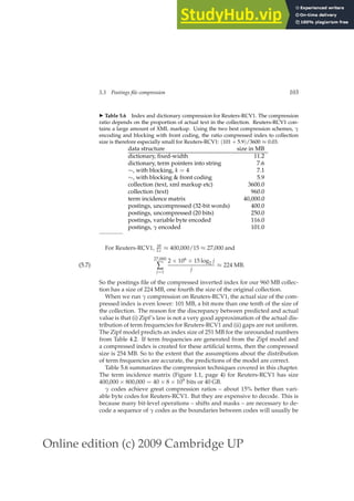
that is either Relevant or Non-relevant. This is illustrated in Figure 6.5, where
seven training examples are shown.
For each training example Φj we have Boolean values sT(dj, qj) and sB(dj, qj)
that we use to compute a score from (6.2)
score(dj, qj) = g · sT(dj, qj) + (1 − g)sB(dj, qj).
(6.3)
We now compare this computed score to the human relevance judgment for
the same document-query pair (dj, qj); to this end, we will quantize each
Relevant judgment as a 1 and each Non-relevant judgment as a 0. Suppose
that we define the error of the scoring function with weight g as
ε(g, Φj) = (r(dj, qj) − score(dj, qj))2
,](https://image.slidesharecdn.com/anintroductiontoinformationretrieval-230807170822-1d67eee0/85/An-Introduction-to-Information-Retrieval-pdf-139-320.jpg)
![Online edition (c) 2009 Cambridge UP
6.1 Parametric and zone indexes 115
Example DocID Query sT sB Judgment
Φ1 37 linux 1 1 Relevant
Φ2 37 penguin 0 1 Non-relevant
Φ3 238 system 0 1 Relevant
Φ4 238 penguin 0 0 Non-relevant
Φ5 1741 kernel 1 1 Relevant
Φ6 2094 driver 0 1 Relevant
Φ7 3191 driver 1 0 Non-relevant
◮ Figure 6.5 An illustration of training examples.
sT sB Score
0 0 0
0 1 1 − g
1 0 g
1 1 1
◮ Figure 6.6 The four possible combinations of sT and sB.
where we have quantized the editorial relevance judgment r(dj, qj) to 0 or 1.
Then, the total error of a set of training examples is given by
∑
j
ε(g, Φj).
(6.4)
The problem of learning the constant g from the given training examples
then reduces to picking the value of g that minimizes the total error in (6.4).
Picking the best value of g in (6.4) in the formulation of Section 6.1.3 re-
duces to the problem of minimizing a quadratic function of g over the inter-
val [0, 1]. This reduction is detailed in Section 6.1.3.
✄ 6.1.3 The optimal weight g
We begin by noting that for any training example Φj for which sT(dj, qj) = 0
and sB(dj, qj) = 1, the score computed by Equation (6.2) is 1 − g. In similar
fashion, we may write down the score computed by Equation (6.2) for the
three other possible combinations of sT(dj, qj) and sB(dj, qj); this is summa-
rized in Figure 6.6.
Let n01r (respectively, n01n) denote the number of training examples for
which sT(dj, qj) = 0 and sB(dj, qj) = 1 and the editorial judgment is Relevant
(respectively, Non-relevant). Then the contribution to the total error in Equa-
tion (6.4) from training examples for which sT(dj, qj) = 0 and sB(dj, qj) = 1](https://image.slidesharecdn.com/anintroductiontoinformationretrieval-230807170822-1d67eee0/85/An-Introduction-to-Information-Retrieval-pdf-140-320.jpg)
![Online edition (c) 2009 Cambridge UP
116 6 Scoring, term weighting and the vector space model
is
[1 − (1 − g)]2
n01r + [0 − (1 − g)]2
n01n.
By writing in similar fashion the error contributions from training examples
of the other three combinations of values for sT(dj, qj) and sB(dj, qj) (and
extending the notation in the obvious manner), the total error corresponding
to Equation (6.4) is
(n01r + n10n)g2
+ (n10r + n01n)(1 − g)2
+ n00r + n11n.
(6.5)
By differentiating Equation (6.5) with respect to g and setting the result to
zero, it follows that the optimal value of g is
n10r + n01n
n10r + n10n + n01r + n01n
.
(6.6)
?
Exercise 6.1
When using weighted zone scoring, is it necessary for all zones to use the same Boo-
lean match function?
Exercise 6.2
In Example 6.1 above with weights g1 = 0.2, g2 = 0.31 and g3 = 0.49, what are all the
distinct score values a document may get?
Exercise 6.3
Rewrite the algorithm in Figure 6.4 to the case of more than two query terms.
Exercise 6.4
Write pseudocode for the function WeightedZone for the case of two postings lists in
Figure 6.4.
Exercise 6.5
Apply Equation 6.6 to the sample training set in Figure 6.5 to estimate the best value
of g for this sample.
Exercise 6.6
For the value of g estimated in Exercise 6.5, compute the weighted zone score for each
(query, document) example. How do these scores relate to the relevance judgments
in Figure 6.5 (quantized to 0/1)?
Exercise 6.7
Why does the expression for g in (6.6) not involve training examples in which sT(dt, qt)
and sB(dt, qt) have the same value?](https://image.slidesharecdn.com/anintroductiontoinformationretrieval-230807170822-1d67eee0/85/An-Introduction-to-Information-Retrieval-pdf-141-320.jpg)


![Online edition (c) 2009 Cambridge UP
6.3 The vector space model for scoring 125
COSINESCORE(q)
1 float Scores[N] = 0
2 Initialize Length[N]
3 for each query term t
4 do calculate wt,q and fetch postings list for t
5 for each pair(d, tft,d) in postings list
6 do Scores[d] += wft,d × wt,q
7 Read the array Length[d]
8 for each d
9 do Scores[d] = Scores[d]/Length[d]
10 return Top K components of Scores[]
◮ Figure 6.14 The basic algorithm for computing vector space scores.
seek the K documents of the collection with the highest vector space scores on
the given query. We now initiate the study of determining the K documents
with the highest vector space scores for a query. Typically, we seek these
K top documents in ordered by decreasing score; for instance many search
engines use K = 10 to retrieve and rank-order the first page of the ten best
results. Here we give the basic algorithm for this computation; we develop a
fuller treatment of efficient techniques and approximations in Chapter 7.
Figure 6.14 gives the basic algorithm for computing vector space scores.
The array Length holds the lengths (normalization factors) for each of the N
documents, whereas the array Scores holds the scores for each of the docu-
ments. When the scores are finally computed in Step 9, all that remains in
Step 10 is to pick off the K documents with the highest scores.
The outermost loop beginning Step 3 repeats the updating of Scores, iter-
ating over each query term t in turn. In Step 5 we calculate the weight in
the query vector for term t. Steps 6-8 update the score of each document by
adding in the contribution from term t. This process of adding in contribu-
tions one query term at a time is sometimes known as term-at-a-time scoring
TERM-AT-A-TIME
or accumulation, and the N elements of the array Scores are therefore known
as accumulators. For this purpose, it would appear necessary to store, with
ACCUMULATOR
each postings entry, the weight wft,d of term t in document d (we have thus
far used either tf or tf-idf for this weight, but leave open the possibility of
other functions to be developed in Section 6.4). In fact this is wasteful, since
storing this weight may require a floating point number. Two ideas help alle-
viate this space problem. First, if we are using inverse document frequency,
we need not precompute idft; it suffices to store N/dft at the head of the
postings for t. Second, we store the term frequency tft,d for each postings en-
try. Finally, Step 12 extracts the top K scores – this requires a priority queue](https://image.slidesharecdn.com/anintroductiontoinformationretrieval-230807170822-1d67eee0/85/An-Introduction-to-Information-Retrieval-pdf-150-320.jpg)


![Online edition (c) 2009 Cambridge UP
136 7 Computing scores in a complete search system
FASTCOSINESCORE(q)
1 float Scores[N] = 0
2 for each d
3 do Initialize Length[d] to the length of doc d
4 for each query term t
5 do calculate wt,q and fetch postings list for t
6 for each pair(d, tft,d) in postings list
7 do add wft,d to Scores[d]
8 Read the array Length[d]
9 for each d
10 do Divide Scores[d] by Length[d]
11 return Top K components of Scores[]
◮ Figure 7.1 A faster algorithm for vector space scores.
two documents d1, d2
~
V(q) ·~
v(d1) ~
V(q) ·~
v(d2) ⇔ ~
v(q) ·~
v(d1) ~
v(q) ·~
v(d2).
(7.1)
For any document d, the cosine similarity ~
V(q) ·~
v(d) is the weighted sum,
over all terms in the query q, of the weights of those terms in d. This in turn
can be computed by a postings intersection exactly as in the algorithm of
Figure 6.14, with line 8 altered since we take wt,q to be 1 so that the multiply-
add in that step becomes just an addition; the result is shown in Figure 7.1.
We walk through the postings in the inverted index for the terms in q, accu-
mulating the total score for each document – very much as in processing a
Boolean query, except we assign a positive score to each document that ap-
pears in any of the postings being traversed. As mentioned in Section 6.3.3
we maintain an idf value for each dictionary term and a tf value for each
postings entry. This scheme computes a score for every document in the
postings of any of the query terms; the total number of such documents may
be considerably smaller than N.
Given these scores, the final step before presenting results to a user is to
pick out the K highest-scoring documents. While one could sort the complete
set of scores, a better approach is to use a heap to retrieve only the top K
documents in order. Where J is the number of documents with non-zero
cosine scores, constructing such a heap can be performed in 2J comparison
steps, following which each of the K highest scoring documents can be “read
off” the heap with log J comparison steps.](https://image.slidesharecdn.com/anintroductiontoinformationretrieval-230807170822-1d67eee0/85/An-Introduction-to-Information-Retrieval-pdf-161-320.jpg)


![Online edition (c) 2009 Cambridge UP
156 8 Evaluation in information retrieval
assumed to have a certain tolerance for seeing some false positives provid-
ing that they get some useful information. The measures of precision and
recall concentrate the evaluation on the return of true positives, asking what
percentage of the relevant documents have been found and how many false
positives have also been returned.
The advantage of having the two numbers for precision and recall is that
one is more important than the other in many circumstances. Typical web
surfers would like every result on the first page to be relevant (high preci-
sion) but have not the slightest interest in knowing let alone looking at every
document that is relevant. In contrast, various professional searchers such as
paralegals and intelligence analysts are very concerned with trying to get as
high recall as possible, and will tolerate fairly low precision results in order to
get it. Individuals searching their hard disks are also often interested in high
recall searches. Nevertheless, the two quantities clearly trade off against one
another: you can always get a recall of 1 (but very low precision) by retriev-
ing all documents for all queries! Recall is a non-decreasing function of the
number of documents retrieved. On the other hand, in a good system, preci-
sion usually decreases as the number of documents retrieved is increased. In
general we want to get some amount of recall while tolerating only a certain
percentage of false positives.
A single measure that trades off precision versus recall is the F measure,
F MEASURE
which is the weighted harmonic mean of precision and recall:
F =
1
α 1
P + (1 − α) 1
R
=
(β2 + 1)PR
β2P + R
where β2
=
1 − α
α
(8.5)
where α ∈ [0, 1] and thus β2 ∈ [0, ∞]. The default balanced F measure equally
weights precision and recall, which means making α = 1/2 or β = 1. It is
commonly written as F1, which is short for Fβ=1, even though the formula-
tion in terms of α more transparently exhibits the F measure as a weighted
harmonic mean. When using β = 1, the formula on the right simplifies to:
Fβ=1 =
2PR
P + R
(8.6)
However, using an even weighting is not the only choice. Values of β 1
emphasize precision, while values of β 1 emphasize recall. For example, a
value of β = 3 or β = 5 might be used if recall is to be emphasized. Recall,
precision, and the F measure are inherently measures between 0 and 1, but
they are also very commonly written as percentages, on a scale between 0
and 100.
Why do we use a harmonic mean rather than the simpler average (arith-
metic mean)? Recall that we can always get 100% recall by just returning all
documents, and therefore we can always get a 50% arithmetic mean by the](https://image.slidesharecdn.com/anintroductiontoinformationretrieval-230807170822-1d67eee0/85/An-Introduction-to-Information-Retrieval-pdf-181-320.jpg)
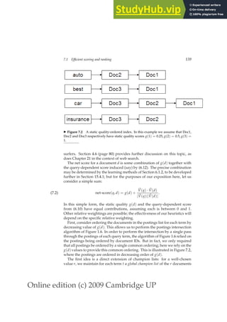
![Online edition (c) 2009 Cambridge UP
8.3 Evaluation of unranked retrieval sets 157
0
2 0
4 0
6 0
8 0
1 0 0
0 2 0 4 0 6 0 8 0 1 0 0
P r e c i s i o n ( R e c a l l f i x e d a t 7 0 % )
M i n i m u m
M a x i m u m
A r i t h m e t i c
G
e o m e t r i c
H a r m o n i c
◮ Figure 8.1 Graph comparing the harmonic mean to other means. The graph
shows a slice through the calculation of various means of precision and recall for
the fixed recall value of 70%. The harmonic mean is always less than either the arith-
metic or geometric mean, and often quite close to the minimum of the two numbers.
When the precision is also 70%, all the measures coincide.
same process. This strongly suggests that the arithmetic mean is an unsuit-
able measure to use. In contrast, if we assume that 1 document in 10,000 is
relevant to the query, the harmonic mean score of this strategy is 0.02%. The
harmonic mean is always less than or equal to the arithmetic mean and the
geometric mean. When the values of two numbers differ greatly, the har-
monic mean is closer to their minimum than to their arithmetic mean; see
Figure 8.1.
?
Exercise 8.1 [⋆]
An IR system returns 8 relevant documents, and 10 nonrelevant documents. There
are a total of 20 relevant documents in the collection. What is the precision of the
system on this search, and what is its recall?
Exercise 8.2 [⋆]
The balanced F measure (a.k.a. F1) is defined as the harmonic mean of precision and
recall. What is the advantage of using the harmonic mean rather than “averaging”
(using the arithmetic mean)?](https://image.slidesharecdn.com/anintroductiontoinformationretrieval-230807170822-1d67eee0/85/An-Introduction-to-Information-Retrieval-pdf-182-320.jpg)
![Online edition (c) 2009 Cambridge UP
158 8 Evaluation in information retrieval
0.0
0.2
0.4
0.6
0.8
1.0
0.0 0.2 0.4 0.6 0.8 1.0
Recall
Precision
◮ Figure 8.2 Precision/recall graph.
Exercise 8.3 [⋆⋆]
Derive the equivalence between the two formulas for F measure shown in Equa-
tion (8.5), given that α = 1/(β2 + 1).
8.4 Evaluation of ranked retrieval results
Precision, recall, and the F measure are set-based measures. They are com-
puted using unordered sets of documents. We need to extend these measures
(or to define new measures) if we are to evaluate the ranked retrieval results
that are now standard with search engines. In a ranked retrieval context,
appropriate sets of retrieved documents are naturally given by the top k re-
trieved documents. For each such set, precision and recall values can be
plotted to give a precision-recall curve, such as the one shown in Figure 8.2.
PRECISION-RECALL
CURVE Precision-recall curves have a distinctive saw-tooth shape: if the (k + 1)th
document retrieved is nonrelevant then recall is the same as for the top k
documents, but precision has dropped. If it is relevant, then both precision
and recall increase, and the curve jags up and to the right. It is often useful to
remove these jiggles and the standard way to do this is with an interpolated
precision: the interpolated precision pinterp at a certain recall level r is defined
INTERPOLATED
PRECISION](https://image.slidesharecdn.com/anintroductiontoinformationretrieval-230807170822-1d67eee0/85/An-Introduction-to-Information-Retrieval-pdf-183-320.jpg)

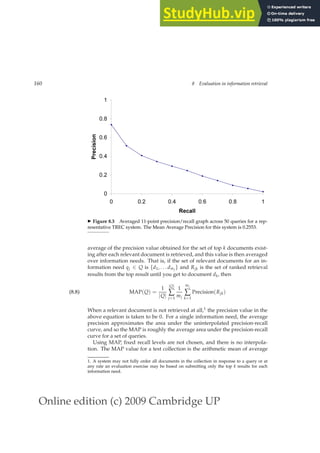
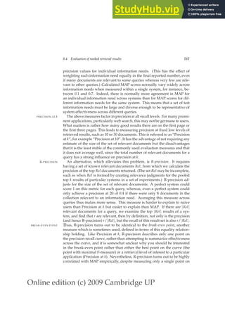

![Online edition (c) 2009 Cambridge UP
8.4 Evaluation of ranked retrieval results 163
lative gain (NDCG). NDCG is designed for situations of non-binary notions
NDCG
of relevance (cf. Section 8.5.1). Like precision at k, it is evaluated over some
number k of top search results. For a set of queries Q, let R(j, d) be the rele-
vance score assessors gave to document d for query j. Then,
NDCG(Q, k) =
1
|Q|
|Q|
∑
j=1
Zkj
k
∑
m=1
2R(j,m) − 1
log2(1 + m)
,
(8.9)
where Zkj is a normalization factor calculated to make it so that a perfect
ranking’s NDCG at k for query j is 1. For queries for which k′ k documents
are retrieved, the last summation is done up to k′.
?
Exercise 8.4 [⋆]
What are the possible values for interpolated precision at a recall level of 0?
Exercise 8.5 [⋆⋆]
Must there always be a break-even point between precision and recall? Either show
there must be or give a counter-example.
Exercise 8.6 [⋆⋆]
What is the relationship between the value of F1 and the break-even point?
Exercise 8.7 [⋆⋆]
The Dice coefficient of two sets is a measure of their intersection scaled by their size
DICE COEFFICIENT
(giving a value in the range 0 to 1):
Dice(X, Y) =
2|X ∩ Y|
|X| + |Y|
Show that the balanced F-measure (F1) is equal to the Dice coefficient of the retrieved
and relevant document sets.
Exercise 8.8 [⋆]
Consider an information need for which there are 4 relevant documents in the collec-
tion. Contrast two systems run on this collection. Their top 10 results are judged for
relevance as follows (the leftmost item is the top ranked search result):
System 1 R N R N N N N N R R
System 2 N R N N R R R N N N
a. What is the MAP of each system? Which has a higher MAP?
b. Does this result intuitively make sense? What does it say about what is important
in getting a good MAP score?
c. What is the R-precision of each system? (Does it rank the systems the same as
MAP?)](https://image.slidesharecdn.com/anintroductiontoinformationretrieval-230807170822-1d67eee0/85/An-Introduction-to-Information-Retrieval-pdf-188-320.jpg)
![Online edition (c) 2009 Cambridge UP
164 8 Evaluation in information retrieval
Exercise 8.9 [⋆⋆]
The following list of Rs and Ns represents relevant (R) and nonrelevant (N) returned
documents in a ranked list of 20 documents retrieved in response to a query from a
collection of 10,000 documents. The top of the ranked list (the document the system
thinks is most likely to be relevant) is on the left of the list. This list shows 6 relevant
documents. Assume that there are 8 relevant documents in total in the collection.
R R N N N N N N R N R N N N R N N N N R
a. What is the precision of the system on the top 20?
b. What is the F1 on the top 20?
c. What is the uninterpolated precision of the system at 25% recall?
d. What is the interpolated precision at 33% recall?
e. Assume that these 20 documents are the complete result set of the system. What
is the MAP for the query?
Assume, now, instead, that the system returned the entire 10,000 documents in a
ranked list, and these are the first 20 results returned.
f. What is the largest possible MAP that this system could have?
g. What is the smallest possible MAP that this system could have?
h. In a set of experiments, only the top 20 results are evaluated by hand. The result
in (e) is used to approximate the range (f)–(g). For this example, how large (in
absolute terms) can the error for the MAP be by calculating (e) instead of (f) and
(g) for this query?
8.5 Assessing relevance
To properly evaluate a system, your test information needs must be germane
to the documents in the test document collection, and appropriate for pre-
dicted usage of the system. These information needs are best designed by
domain experts. Using random combinations of query terms as an informa-
tion need is generally not a good idea because typically they will not resem-
ble the actual distribution of information needs.
Given information needs and documents, you need to collect relevance
assessments. This is a time-consuming and expensive process involving hu-
man beings. For tiny collections like Cranfield, exhaustive judgments of rel-
evance for each query and document pair were obtained. For large modern
collections, it is usual for relevance to be assessed only for a subset of the
documents for each query. The most standard approach is pooling, where rel-
POOLING
evance is assessed over a subset of the collection that is formed from the top
k documents returned by a number of different IR systems (usually the ones
to be evaluated), and perhaps other sources such as the results of Boolean
keyword searches or documents found by expert searchers in an interactive
process.](https://image.slidesharecdn.com/anintroductiontoinformationretrieval-230807170822-1d67eee0/85/An-Introduction-to-Information-Retrieval-pdf-189-320.jpg)
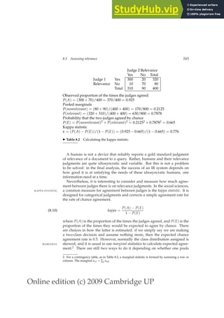

![Online edition (c) 2009 Cambridge UP
8.5 Assessing relevance 167
and machine learning methods for adjusting parameter weights in scoring
(Section 6.1.2).
That is not to say that there are not problems latent within the abstrac-
tions used. The relevance of one document is treated as independent of the
relevance of other documents in the collection. (This assumption is actually
built into most retrieval systems – documents are scored against queries, not
against each other – as well as being assumed in the evaluation methods.)
Assessments are binary: there aren’t any nuanced assessments of relevance.
Relevance of a document to an information need is treated as an absolute,
objective decision. But judgments of relevance are subjective, varying across
people, as we discussed above. In practice, human assessors are also imper-
fect measuring instruments, susceptible to failures of understanding and at-
tention. We also have to assume that users’ information needs do not change
as they start looking at retrieval results. Any results based on one collection
are heavily skewed by the choice of collection, queries, and relevance judg-
ment set: the results may not translate from one domain to another or to a
different user population.
Some of these problems may be fixable. A number of recent evaluations,
including INEX, some TREC tracks, and NTCIR have adopted an ordinal
notion of relevance with documents divided into 3 or 4 classes, distinguish-
ing slightly relevant documents from highly relevant documents. See Sec-
tion 10.4 (page 210) for a detailed discussion of how this is implemented in
the INEX evaluations.
One clear problem with the relevance-based assessment that we have pre-
sented is the distinction between relevance and marginal relevance: whether
MARGINAL RELEVANCE
a document still has distinctive usefulness after the user has looked at cer-
tain other documents (Carbonell and Goldstein 1998). Even if a document
is highly relevant, its information can be completely redundant with other
documents which have already been examined. The most extreme case of
this is documents that are duplicates – a phenomenon that is actually very
common on the World Wide Web – but it can also easily occur when sev-
eral documents provide a similar precis of an event. In such circumstances,
marginal relevance is clearly a better measure of utility to the user. Maximiz-
ing marginal relevance requires returning documents that exhibit diversity
and novelty. One way to approach measuring this is by using distinct facts
or entities as evaluation units. This perhaps more directly measures true
utility to the user but doing this makes it harder to create a test collection.
? Exercise 8.10 [⋆⋆]
Below is a table showing how two human judges rated the relevance of a set of 12
documents to a particular information need (0 = nonrelevant, 1 = relevant). Let us as-
sume that you’ve written an IR system that for this query returns the set of documents
{4, 5, 6, 7, 8}.](https://image.slidesharecdn.com/anintroductiontoinformationretrieval-230807170822-1d67eee0/85/An-Introduction-to-Information-Retrieval-pdf-192-320.jpg)


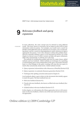
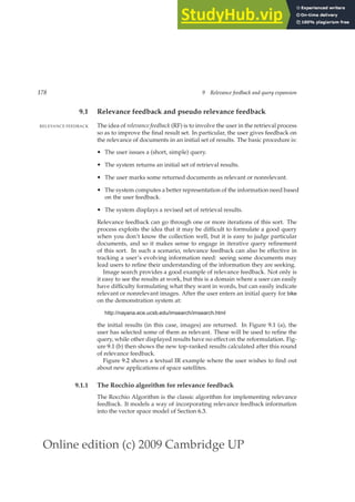


![Online edition (c) 2009 Cambridge UP
9.1 Relevance feedback and pseudo relevance feedback 181
◮ Figure 9.3 The Rocchio optimal query for separating relevant and nonrelevant
documents.
The underlying theory. We want to find a query vector, denoted as ~
q, that
maximizes similarity with relevant documents while minimizing similarity
with nonrelevant documents. If Cr is the set of relevant documents and Cnr
is the set of nonrelevant documents, then we wish to find:1
~
qopt = arg max
~
q
[sim(~
q, Cr) − sim(~
q, Cnr)],
(9.1)
where sim is defined as in Equation 6.10. Under cosine similarity, the optimal
query vector~
qopt for separating the relevant and nonrelevant documents is:
~
qopt =
1
|Cr| ∑
~
dj∈Cr
~
dj −
1
|Cnr| ∑
~
dj∈Cnr
~
dj
(9.2)
That is, the optimal query is the vector difference between the centroids of the
relevant and nonrelevant documents; see Figure 9.3. However, this observa-
tion is not terribly useful, precisely because the full set of relevant documents
is not known: it is what we want to find.
The Rocchio (1971) algorithm. This was the relevance feedback mecha-
ROCCHIO ALGORITHM
1. In the equation, arg maxx f (x) returns a value of x which maximizes the value of the function
f (x). Similarly, arg minx f (x) returns a value of x which minimizes the value of the function
f (x).](https://image.slidesharecdn.com/anintroductiontoinformationretrieval-230807170822-1d67eee0/85/An-Introduction-to-Information-Retrieval-pdf-206-320.jpg)
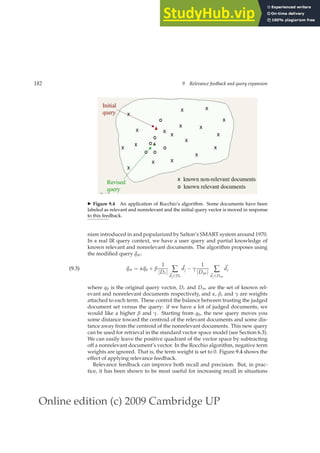

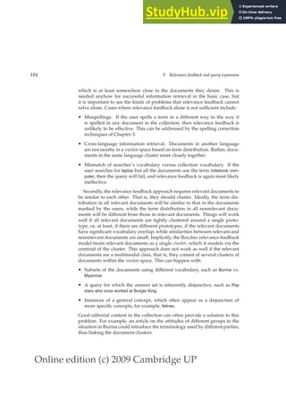
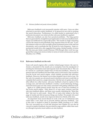
![Online edition (c) 2009 Cambridge UP
186 9 Relevance feedback and query expansion
? Exercise 9.1
In Rocchio’s algorithm, what weight setting for α/β/γ does a “Find pages like this
one” search correspond to?
Exercise 9.2 [⋆]
Give three reasons why relevance feedback has been little used in web search.
9.1.5 Evaluation of relevance feedback strategies
Interactive relevance feedback can give very substantial gains in retrieval
performance. Empirically, one round of relevance feedback is often very
useful. Two rounds is sometimes marginally more useful. Successful use of
relevance feedback requires enough judged documents, otherwise the pro-
cess is unstable in that it may drift away from the user’s information need.
Accordingly, having at least five judged documents is recommended.
There is some subtlety to evaluating the effectiveness of relevance feed-
back in a sound and enlightening way. The obvious first strategy is to start
with an initial query q0 and to compute a precision-recall graph. Following
one round of feedback from the user, we compute the modified query qm
and again compute a precision-recall graph. Here, in both rounds we assess
performance over all documents in the collection, which makes comparisons
straightforward. If we do this, we find spectacular gains from relevance feed-
back: gains on the order of 50% in mean average precision. But unfortunately
it is cheating. The gains are partly due to the fact that known relevant doc-
uments (judged by the user) are now ranked higher. Fairness demands that
we should only evaluate with respect to documents not seen by the user.
A second idea is to use documents in the residual collection (the set of doc-
uments minus those assessed relevant) for the second round of evaluation.
This seems like a more realistic evaluation. Unfortunately, the measured per-
formance can then often be lower than for the original query. This is partic-
ularly the case if there are few relevant documents, and so a fair proportion
of them have been judged by the user in the first round. The relative per-
formance of variant relevance feedback methods can be validly compared,
but it is difficult to validly compare performance with and without relevance
feedback because the collection size and the number of relevant documents
changes from before the feedback to after it.
Thus neither of these methods is fully satisfactory. A third method is to
have two collections, one which is used for the initial query and relevance
judgments, and the second that is then used for comparative evaluation. The
performance of both q0 and qm can be validly compared on the second col-
lection.
Perhaps the best evaluation of the utility of relevance feedback is to do user
studies of its effectiveness, in particular by doing a time-based comparison:](https://image.slidesharecdn.com/anintroductiontoinformationretrieval-230807170822-1d67eee0/85/An-Introduction-to-Information-Retrieval-pdf-211-320.jpg)

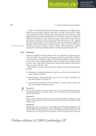
![Online edition (c) 2009 Cambridge UP
9.2 Global methods for query reformulation 189
frequency). There is no need to length-normalize vectors. Using Rocchio relevance
feedback as in Equation (9.3) what would the revised query vector be after relevance
feedback? Assume α = 1, β = 0.75, γ = 0.25.
Exercise 9.6 [⋆]
Omar has implemented a relevance feedback web search system, where he is going
to do relevance feedback based only on words in the title text returned for a page (for
efficiency). The user is going to rank 3 results. The first user, Jinxing, queries for:
banana slug
and the top three titles returned are:
banana slug Ariolimax columbianus
Santa Cruz mountains banana slug
Santa Cruz Campus Mascot
Jinxing judges the first two documents relevant, and the third nonrelevant. Assume
that Omar’s search engine uses term frequency but no length normalization nor IDF.
Assume that he is using the Rocchio relevance feedback mechanism, with α = β =
γ = 1. Show the final revised query that would be run. (Please list the vector elements
in alphabetical order.)
9.2 Global methods for query reformulation
In this section we more briefly discuss three global methods for expanding a
query: by simply aiding the user in doing so, by using a manual thesaurus,
and through building a thesaurus automatically.
9.2.1 Vocabulary tools for query reformulation
Various user supports in the search process can help the user see how their
searches are or are not working. This includes information about words that
were omitted from the query because they were on stop lists, what words
were stemmed to, the number of hits on each term or phrase, and whether
words were dynamically turned into phrases. The IR system might also sug-
gest search terms by means of a thesaurus or a controlled vocabulary. A user
can also be allowed to browse lists of the terms that are in the inverted index,
and thus find good terms that appear in the collection.
9.2.2 Query expansion
In relevance feedback, users give additional input on documents (by mark-
ing documents in the results set as relevant or not), and this input is used
to reweight the terms in the query for documents. In query expansion on the
QUERY EXPANSION
other hand, users give additional input on query words or phrases, possibly
suggesting additional query terms. Some search engines (especially on the](https://image.slidesharecdn.com/anintroductiontoinformationretrieval-230807170822-1d67eee0/85/An-Introduction-to-Information-Retrieval-pdf-214-320.jpg)
![Online edition (c) 2009 Cambridge UP
190 9 Relevance feedback and query expansion
Y a h o o ! M y Y a h o o ! M a i l W e l c o m e , G u e s t [ S i g n I n ] H e l p
S e a r c h
p a l m
W
e b I m a g e s V i d e o L o c a l S h o p p i n g m o r e
O p t i o n s
A l s o t r y :
S P O N S O R R E S U L T S
p a
l m t r e e s ,
p a
l m s p r i n g s ,
p a
l m c e n t r o ,
p a
l m
t r e o , M o r e . . .
P
a
l m ❜ A T T
a t t . c o m / w i r e l e s s ❧ G o m o b i l e e f f o r t l e s s l y w i t h t h e P A L M T r e o f r o m
A
T T ( C i n g u l a r ) .
P
a
l m H a n d h e l d s
P a l m . c o m ❧ O r g a n i z e r , P l a n n e r , W i F i , M u s i c B l u e t o o t h , G a m e s ,
P h o t o s V i d e o .
P
a
l m , I n c .
M a k e r o f h a n d h e l d P D
A
d e v i c e s t h a t a l l o w m o b i l e u s e r s t o m a n a g e
s c h e d u l e s , c o n t a c t s , a n d o t h e r p e r s o n a l a n d b u s i n e s s i n f o r m a t i o n .
w w w . p a l m . c o m ❧ C a c h e d
P
a
l m , I n c . ❜ T r e o a n d C e n t r o s m a r t p h o n e s , h a n d h e l d s ,
a n d a c c e s s o r i e s
P a l m , I n c . , i n n o v a t o r o f e a s y ❧ t o ❧ u s e m o b i l e p r o d u c t s i n c l u d i n g
P a l m ® T r e o _ a n d C e n t r o _ s m a r t p h o n e s , P a l m h a n d h e l d s , s e r v i c e s ,
a n d a c c e s s o r i e s .
w w w . p a l m . c o m / u s ❧ C a c h e d
S P O N S O R R E S U L T S
H a n d h e l d s a t D e l l
S t a y C o n n e c t e d w i t h
H
a n d h e l d P C s P D
A
s .
S h o p a t D e l l ™ O f f i c i a l
S i t e .
w w w . D e l l . c o m
B u y P
a
l m C e n t r o
C a s e s
U
l t i m a t e s e l e c t i o n o f
c a s e s a n d a c c e s s o r i e s
f o r b u s i n e s s d e v i c e s .
w w w . C a s e s . c o m
F r e e P l a m T r e o
G e t
A
F r e e P a l m T r e o
7 0 0
W P h o n e . P a r t i c i p a t e
T o d a y .
E v
a l u a t i o n N a t i o n . c o m /
t r e o
1 ➟ 1 0
o f a b o u t 5 3 4 ,
0 0 0
,
0 0 0
f o r p a l m ( A b o u t t h i s p a g e )
➟ 0 . 1 1
s e c
.
◮ Figure 9.6 An example of query expansion in the interface of the Yahoo! web
search engine in 2006. The expanded query suggestions appear just below the “Search
Results” bar.
web) suggest related queries in response to a query; the users then opt to use
one of these alternative query suggestions. Figure 9.6 shows an example of
query suggestion options being presented in the Yahoo! web search engine.
The central question in this form of query expansion is how to generate al-
ternative or expanded queries for the user. The most common form of query
expansion is global analysis, using some form of thesaurus. For each term
t in a query, the query can be automatically expanded with synonyms and
related words of t from the thesaurus. Use of a thesaurus can be combined
with ideas of term weighting: for instance, one might weight added terms
less than original query terms.
Methods for building a thesaurus for query expansion include:
• Use of a controlled vocabulary that is maintained by human editors. Here,
there is a canonical term for each concept. The subject headings of tra-
ditional library subject indexes, such as the Library of Congress Subject
Headings, or the Dewey Decimal system are examples of a controlled
vocabulary. Use of a controlled vocabulary is quite common for well-
resourced domains. A well-known example is the Unified Medical Lan-
guage System (UMLS) used with MedLine for querying the biomedical
research literature. For example, in Figure 9.7, neoplasms was added to a](https://image.slidesharecdn.com/anintroductiontoinformationretrieval-230807170822-1d67eee0/85/An-Introduction-to-Information-Retrieval-pdf-215-320.jpg)
![Online edition (c) 2009 Cambridge UP
9.2 Global methods for query reformulation 191
• User query: cancer
• PubMed query: (“neoplasms”[TIAB] NOT Medline[SB]) OR “neoplasms”[MeSH
Terms] OR cancer[Text Word]
• User query: skin itch
• PubMed query: (“skin”[MeSH Terms] OR (“integumentary system”[TIAB] NOT
Medline[SB]) OR “integumentary system”[MeSH Terms] OR skin[Text Word]) AND
((“pruritus”[TIAB] NOT Medline[SB]) OR “pruritus”[MeSH Terms] OR itch[Text
Word])
◮ Figure 9.7 Examples of query expansion via the PubMed thesaurus. When a user
issues a query on the PubMed interface to Medline at http://www.ncbi.nlm.nih.gov/entrez/,
their query is mapped on to the Medline vocabulary as shown.
search for cancer. This Medline query expansion also contrasts with the
Yahoo! example. The Yahoo! interface is a case of interactive query expan-
sion, whereas PubMed does automatic query expansion. Unless the user
chooses to examine the submitted query, they may not even realize that
query expansion has occurred.
• A manual thesaurus. Here, human editors have built up sets of synony-
mous names for concepts, without designating a canonical term. The
UMLS metathesaurus is one example of a thesaurus. Statistics Canada
maintains a thesaurus of preferred terms, synonyms, broader terms, and
narrower terms for matters on which the government collects statistics,
such as goods and services. This thesaurus is also bilingual English and
French.
• An automatically derived thesaurus. Here, word co-occurrence statistics
over a collection of documents in a domain are used to automatically in-
duce a thesaurus; see Section 9.2.3.
• Query reformulations based on query log mining. Here, we exploit the
manual query reformulations of other users to make suggestions to a new
user. This requires a huge query volume, and is thus particularly appro-
priate to web search.
Thesaurus-based query expansion has the advantage of not requiring any
user input. Use of query expansion generally increases recall and is widely
used in many science and engineering fields. As well as such global analysis
techniques, it is also possible to do query expansion by local analysis, for
instance, by analyzing the documents in the result set. User input is now](https://image.slidesharecdn.com/anintroductiontoinformationretrieval-230807170822-1d67eee0/85/An-Introduction-to-Information-Retrieval-pdf-216-320.jpg)
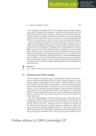

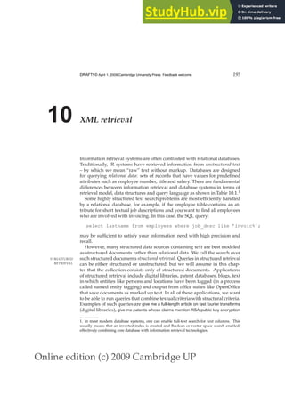


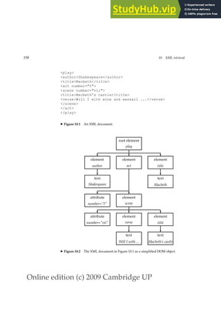
![Online edition (c) 2009 Cambridge UP
10.1 Basic XML concepts 199
//article
[.//yr = 2001 or .//yr = 2002]
//section
[about(.,summer holidays)]
holidays
summer
section
article
◮ Figure 10.3 An XML query in NEXI format and its partial representation as a tree.
can process an XML document by starting at the root element and then de-
scending down the tree from parents to children.
XPath is a standard for enumerating paths in an XML document collection.
XPATH
We will also refer to paths as XML contexts or simply contexts in this chapter.
XML CONTEXT
Only a small subset of XPath is needed for our purposes. The XPath expres-
sion node selects all nodes of that name. Successive elements of a path are
separated by slashes, so act/scene selects all scene elements whose par-
ent is an act element. Double slashes indicate that an arbitrary number of
elements can intervene on a path: play//scene selects all scene elements
occurring in a play element. In Figure 10.2 this set consists of a single scene el-
ement, which is accessible via the path play, act, scene from the top. An initial
slash starts the path at the root element. /play/title selects the play’s ti-
tle in Figure 10.1, /play//title selects a set with two members (the play’s
title and the scene’s title), and /scene/title selects no elements. For no-
tational convenience, we allow the final element of a path to be a vocabulary
term and separate it from the element path by the symbol #, even though this
does not conform to the XPath standard. For example, title#Macbeth
selects all titles containing the term Macbeth.
We also need the concept of schema in this chapter. A schema puts con-
SCHEMA
straints on the structure of allowable XML documents for a particular ap-
plication. A schema for Shakespeare’s plays may stipulate that scenes can
only occur as children of acts and that only acts and scenes have the num-
ber attribute. Two standards for schemas for XML documents are XML DTD
XML DTD
(document type definition) and XML Schema. Users can only write structured
XML SCHEMA
queries for an XML retrieval system if they have some minimal knowledge
about the schema of the collection.
root node and text is not embedded in text nodes. See http://www.w3.org/DOM/.](https://image.slidesharecdn.com/anintroductiontoinformationretrieval-230807170822-1d67eee0/85/An-Introduction-to-Information-Retrieval-pdf-224-320.jpg)
![Online edition (c) 2009 Cambridge UP
200 10 XML retrieval
M’s castle
title
Will I . . .
verse
scene
Julius Caesar
title
book
Gallic war
title
Julius Caesar
author
book
d1 q1 q2
◮ Figure 10.4 Tree representation of XML documents and queries.
A common format for XML queries is NEXI (Narrowed Extended XPath
NEXI
I). We give an example in Figure 10.3. We display the query on four lines for
typographical convenience, but it is intended to be read as one unit without
line breaks. In particular, //section is embedded under //article.
The query in Figure 10.3 specifies a search for sections about the sum-
mer holidays that are part of articles from 2001 or 2002. As in XPath dou-
ble slashes indicate that an arbitrary number of elements can intervene on
a path. The dot in a clause in square brackets refers to the element the
clause modifies. The clause [.//yr = 2001 or .//yr = 2002] mod-
ifies //article. Thus, the dot refers to //article in this case. Similarly,
the dot in [about(., summer holidays)] refers to the section that the
clause modifies.
The two yr conditions are relational attribute constraints. Only articles
whose yr attribute is 2001 or 2002 (or that contain an element whose yr
attribute is 2001 or 2002) are to be considered. The about clause is a ranking
constraint: Sections that occur in the right type of article are to be ranked
according to how relevant they are to the topic summer holidays.
We usually handle relational attribute constraints by prefiltering or post-
filtering: We simply exclude all elements from the result set that do not meet
the relational attribute constraints. In this chapter, we will not address how
to do this efficiently and instead focus on the core information retrieval prob-
lem in XML retrieval, namely how to rank documents according to the rele-
vance criteria expressed in the about conditions of the NEXI query.
If we discard relational attributes, we can represent documents as trees
with only one type of node: element nodes. In other words, we remove
all attribute nodes from the XML document, such as the number attribute in
Figure 10.1. Figure 10.4 shows a subtree of the document in Figure 10.1 as an
element-node tree (labeled d1).](https://image.slidesharecdn.com/anintroductiontoinformationretrieval-230807170822-1d67eee0/85/An-Introduction-to-Information-Retrieval-pdf-225-320.jpg)

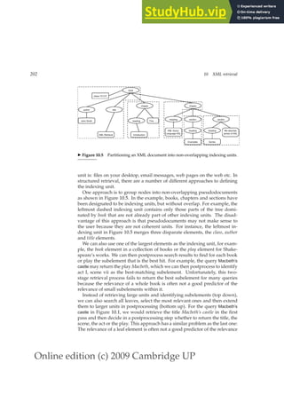


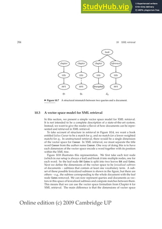
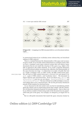

![Online edition (c) 2009 Cambridge UP
10.3 A vector space model for XML retrieval 209
SCOREDOCUMENTSWITHSIMNOMERGE(q, B, V, N, normalizer)
1 for n ← 1 to N
2 do score[n] ← 0
3 for each hcq, ti ∈ q
4 do wq ← WEIGHT(q, t, cq)
5 for each c ∈ B
6 do if CR(cq, c) 0
7 then postings ← GETPOSTINGS(hc, ti)
8 for each posting ∈ postings
9 do x ← CR(cq, c) ∗ wq ∗ weight(posting)
10 score[docID(posting)] += x
11 for n ← 1 to N
12 do score[n] ← score[n]/normalizer[n]
13 return score
◮ Figure 10.9 The algorithm for scoring documents with SIMNOMERGE.
query
hc1, ti
CR(c1, c1)=1.0
CR(c1, c2)=0
CR(c1, c3)=0.63
inverted index
hc1, ti −→ hd1, 0.5i hd4, 0.1i hd9, 0.2i ...
hc2, ti −→ hd2, 0.25i hd3, 0.1i hd12, 0.9i ...
hc3, ti −→ hd3, 0.7i hd6, 0.8i hd9, 0.6i ...
◮ Figure 10.10 Scoring of a query with one structural term in SIMNOMERGE.
next context has no context resemblance with c1: CR(c1, c2) = 0 and the cor-
responding postings list is ignored. The context match of c1 with c3 is 0.630
and it will be processed. In this example, the highest ranking document is d9
with a similarity of 1.0 × 0.2 + 0.63 × 0.6 = 0.578. To simplify the figure, the
query weight of hc1, ti is assumed to be 1.0.
The query-document similarity function in Figure 10.9 is called SIMNOMERGE
because different XML contexts are kept separate for the purpose of weight-
ing. An alternative similarity function is SIMMERGE which relaxes the match-
ing conditions of query and document further in the following three ways.](https://image.slidesharecdn.com/anintroductiontoinformationretrieval-230807170822-1d67eee0/85/An-Introduction-to-Information-Retrieval-pdf-234-320.jpg)
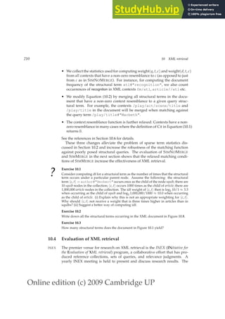
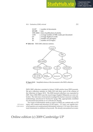
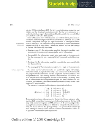
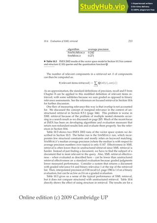

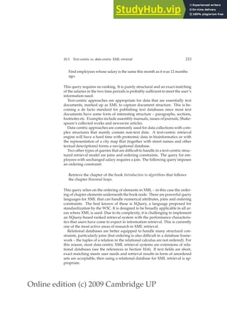

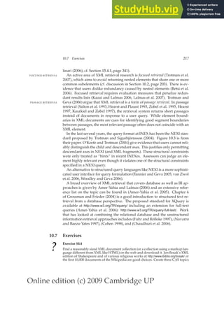

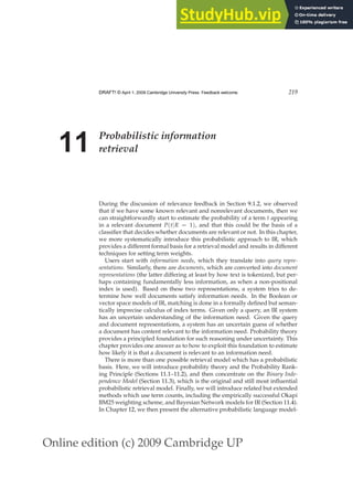
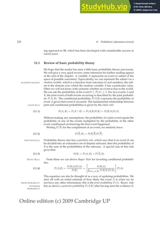


![Online edition (c) 2009 Cambridge UP
11.3 The Binary Independence Model 227
α = 1
2. This is a form of maximum a posteriori (MAP) estimation, where we
MAXIMUM A
POSTERIORI
MAP
choose the most likely point value for probabilities based on the prior and
the observed evidence, following Equation (11.4). We will further discuss
methods of smoothing estimated counts to give probability models in Sec-
tion 12.2.2 (page 243); the simple method of adding 1
2 to each observed count
will do for now.
11.3.3 Probability estimates in practice
Under the assumption that relevant documents are a very small percentage
of the collection, it is plausible to approximate statistics for nonrelevant doc-
uments by statistics from the whole collection. Under this assumption, ut
(the probability of term occurrence in nonrelevant documents for a query) is
dft/N and
log[(1 − ut)/ut] = log[(N − dft)/dft] ≈ log N/dft
(11.22)
In other words, we can provide a theoretical justification for the most fre-
quently used form of idf weighting, which we saw in Section 6.2.1.
The approximation technique in Equation (11.22) cannot easily be extended
to relevant documents. The quantity pt can be estimated in various ways:
1. We can use the frequency of term occurrence in known relevant docu-
ments (if we know some). This is the basis of probabilistic approaches to
relevance feedback weighting in a feedback loop, discussed in the next
subsection.
2. Croft and Harper (1979) proposed using a constant in their combination
match model. For instance, we might assume that pt is constant over all
terms xt in the query and that pt = 0.5. This means that each term has
even odds of appearing in a relevant document, and so the pt and (1 − pt)
factors cancel out in the expression for RSV. Such an estimate is weak, but
doesn’t disagree violently with our hopes for the search terms appearing
in many but not all relevant documents. Combining this method with our
earlier approximation for ut, the document ranking is determined simply
by which query terms occur in documents scaled by their idf weighting.
For short documents (titles or abstracts) in situations in which iterative
searching is undesirable, using this weighting term alone can be quite
satisfactory, although in many other circumstances we would like to do
better.
3. Greiff (1998) argues that the constant estimate of pt in the Croft and Harper
(1979) model is theoretically problematic and not observed empirically: as
might be expected, pt is shown to rise with dft. Based on his data analysis,
a plausible proposal would be to use the estimate pt = 1
3 + 2
3 dft/N.](https://image.slidesharecdn.com/anintroductiontoinformationretrieval-230807170822-1d67eee0/85/An-Introduction-to-Information-Retrieval-pdf-252-320.jpg)

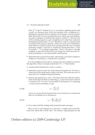
![Online edition (c) 2009 Cambridge UP
230 11 Probabilistic information retrieval
Equation (11.22), and Equation (11.26), we have:
ct = log
pt
1 − pt
·
1 − ut
ut
≈ log
|Vt| + 1
2
|V| − |Vt| + 1
·
N
dft
#
(11.28)
But things aren’t quite the same: pt/(1 − pt) measures the (estimated) pro-
portion of relevant documents that the term t occurs in, not term frequency.
Moreover, if we apply log identities:
ct = log
|Vt| + 1
2
|V| − |Vt| + 1
+ log
N
dft
(11.29)
we see that we are now adding the two log scaled components rather than
multiplying them.
?
Exercise 11.1
Work through the derivation of Equation (11.20) from Equations (11.18) and (11.19).
Exercise 11.2
What are the differences between standard vector space tf-idf weighting and the BIM
probabilistic retrieval model (in the case where no document relevance information
is available)?
Exercise 11.3 [⋆⋆]
Let Xt be a random variable indicating whether the term t appears in a document.
Suppose we have |R| relevant documents in the document collection and that Xt = 1
in s of the documents. Take the observed data to be just these observations of Xt for
each document in R. Show that the MLE for the parameter pt = P(Xt = 1|R = 1,~
q),
that is, the value for pt which maximizes the probability of the observed data, is
pt = s/|R|.
Exercise 11.4
Describe the differences between vector space relevance feedback and probabilistic
relevance feedback.
11.4 An appraisal and some extensions
11.4.1 An appraisal of probabilistic models
Probabilistic methods are one of the oldest formal models in IR. Already
in the 1970s they were held out as an opportunity to place IR on a firmer
theoretical footing, and with the resurgence of probabilistic methods in com-
putational linguistics in the 1990s, that hope has returned, and probabilis-
tic methods are again one of the currently hottest topics in IR. Traditionally,
probabilistic IR has had neat ideas but the methods have never won on per-
formance. Getting reasonable approximations of the needed probabilities for](https://image.slidesharecdn.com/anintroductiontoinformationretrieval-230807170822-1d67eee0/85/An-Introduction-to-Information-Retrieval-pdf-255-320.jpg)
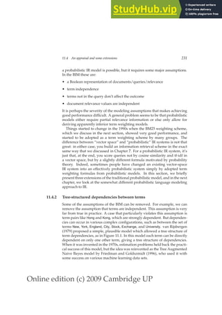
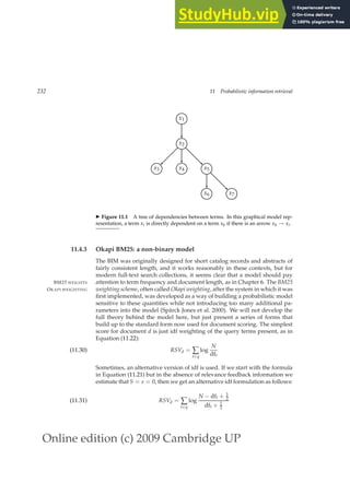


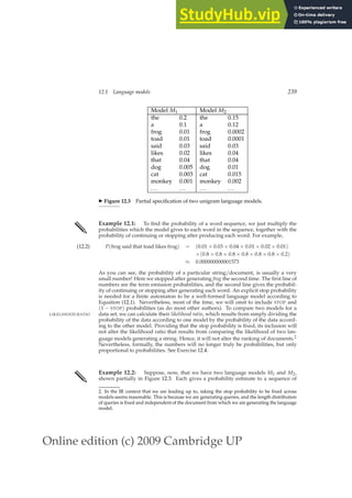

![Online edition (c) 2009 Cambridge UP
242 12 Language models for information retrieval
different sequences, which we have never observed before, and so the model
has to generalize beyond the observed data to allow unknown words and se-
quences. This interpretation is not so clear in the IR case, where a document
is finite and usually fixed. The strategy we adopt in IR is as follows. We
pretend that the document d is only a representative sample of text drawn
from a model distribution, treating it like a fine-grained topic. We then esti-
mate a language model from this sample, and use that model to calculate the
probability of observing any word sequence, and, finally, we rank documents
according to their probability of generating the query.
?
Exercise 12.1 [⋆]
Including stop probabilities in the calculation, what will the sum of the probability
estimates of all strings in the language of length 1 be? Assume that you generate a
word and then decide whether to stop or not (i.e., the null string is not part of the
language).
Exercise 12.2 [⋆]
If the stop probability is omitted from calculations, what will the sum of the scores
assigned to strings in the language of length 1 be?
Exercise 12.3 [⋆]
What is the likelihood ratio of the document according to M1 and M2 in Exam-
ple 12.2?
Exercise 12.4 [⋆]
No explicit STOP probability appeared in Example 12.2. Assuming that the STOP
probability of each model is 0.1, does this change the likelihood ratio of a document
according to the two models?
Exercise 12.5 [⋆⋆]
How might a language model be used in a spelling correction system? In particular,
consider the case of context-sensitive spelling correction, and correcting incorrect us-
ages of words, such as their in Are you their? (See Section 3.5 (page 65) for pointers to
some literature on this topic.)
12.2 The query likelihood model
12.2.1 Using query likelihood language models in IR
Language modeling is a quite general formal approach to IR, with many vari-
ant realizations. The original and basic method for using language models
in IR is the query likelihood model. In it, we construct from each document d
QUERY LIKELIHOOD
MODEL in the collection a language model Md. Our goal is to rank documents by
P(d|q), where the probability of a document is interpreted as the likelihood
that it is relevant to the query. Using Bayes rule (as introduced in Section 11.1,
page 220), we have:
P(d|q) = P(q|d)P(d)/P(q)](https://image.slidesharecdn.com/anintroductiontoinformationretrieval-230807170822-1d67eee0/85/An-Introduction-to-Information-Retrieval-pdf-267-320.jpg)
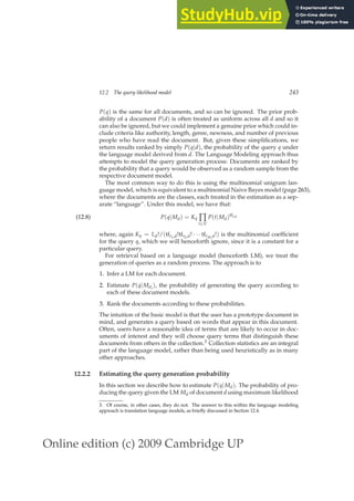

![Online edition (c) 2009 Cambridge UP
246 12 Language models for information retrieval
of the models. The reason for this is explored in Exercise 12.8. The extent
of smoothing in these two models is controlled by the λ and α parameters: a
small value of λ or a large value of α means more smoothing. This parameter
can be tuned to optimize performance using a line search (or, for the linear
interpolation model, by other methods, such as the expectation maximimiza-
tion algorithm; see Section 16.5, page 368). The value need not be a constant.
One approach is to make the value a function of the query size. This is useful
because a small amount of smoothing (a “conjunctive-like” search) is more
suitable for short queries, while a lot of smoothing is more suitable for long
queries.
To summarize, the retrieval ranking for a query q under the basic LM for
IR we have been considering is given by:
P(d|q) ∝ P(d) ∏
t∈q
((1 − λ)P(t|Mc) + λP(t|Md))
(12.12)
This equation captures the probability that the document that the user had
in mind was in fact d.
✎ Example 12.3: Suppose the document collection contains two documents:
• d1: Xyzzy reports a profit but revenue is down
• d2: Quorus narrows quarter loss but revenue decreases further
The model will be MLE unigram models from the documents and collection, mixed
with λ = 1/2.
Suppose the query is revenue down. Then:
P(q|d1) = [(1/8 + 2/16)/2] × [(1/8 + 1/16)/2]
(12.13)
= 1/8 × 3/32 = 3/256
P(q|d2) = [(1/8 + 2/16)/2] × [(0/8 + 1/16)/2]
= 1/8 × 1/32 = 1/256
So, the ranking is d1 d2.
12.2.3 Ponte and Croft’s Experiments
Ponte and Croft (1998) present the first experiments on the language model-
ing approach to information retrieval. Their basic approach is the model that
we have presented until now. However, we have presented an approach
where the language model is a mixture of two multinomials, much as in
(Miller et al. 1999, Hiemstra 2000) rather than Ponte and Croft’s multivari-
ate Bernoulli model. The use of multinomials has been standard in most
subsequent work in the LM approach and experimental results in IR, as
well as evidence from text classification which we consider in Section 13.3](https://image.slidesharecdn.com/anintroductiontoinformationretrieval-230807170822-1d67eee0/85/An-Introduction-to-Information-Retrieval-pdf-271-320.jpg)
![Online edition (c) 2009 Cambridge UP
12.2 The query likelihood model 247
Precision
Rec. tf-idf LM %chg
0.0 0.7439 0.7590 +2.0
0.1 0.4521 0.4910 +8.6
0.2 0.3514 0.4045 +15.1 *
0.3 0.2761 0.3342 +21.0 *
0.4 0.2093 0.2572 +22.9 *
0.5 0.1558 0.2061 +32.3 *
0.6 0.1024 0.1405 +37.1 *
0.7 0.0451 0.0760 +68.7 *
0.8 0.0160 0.0432 +169.6 *
0.9 0.0033 0.0063 +89.3
1.0 0.0028 0.0050 +76.9
Ave 0.1868 0.2233 +19.55 *
◮ Figure 12.4 Results of a comparison of tf-idf with language modeling (LM) term
weighting by Ponte and Croft (1998). The version of tf-idf from the INQUERY IR sys-
tem includes length normalization of tf. The table gives an evaluation according to
11-point average precision with significance marked with a * according to a Wilcoxon
signed rank test. The language modeling approach always does better in these exper-
iments, but note that where the approach shows significant gains is at higher levels
of recall.
(page 263), suggests that it is superior. Ponte and Croft argued strongly for
the effectiveness of the term weights that come from the language modeling
approach over traditional tf-idf weights. We present a subset of their results
in Figure 12.4 where they compare tf-idf to language modeling by evaluating
TREC topics 202–250 over TREC disks 2 and 3. The queries are sentence-
length natural language queries. The language modeling approach yields
significantly better results than their baseline tf-idf based term weighting ap-
proach. And indeed the gains shown here have been extended in subsequent
work.
? Exercise 12.6 [⋆]
Consider making a language model from the following training text:
the martian has landed on the latin pop sensation ricky martin
a. Under a MLE-estimated unigram probability model, what are P(the) and P(martian)?
b. Under a MLE-estimated bigram model, what are P(sensation|pop) and P(pop|the)?](https://image.slidesharecdn.com/anintroductiontoinformationretrieval-230807170822-1d67eee0/85/An-Introduction-to-Information-Retrieval-pdf-272-320.jpg)
![Online edition (c) 2009 Cambridge UP
248 12 Language models for information retrieval
Exercise 12.7 [⋆⋆]
Suppose we have a collection that consists of the 4 documents given in the below
table.
docID Document text
1 click go the shears boys click click click
2 click click
3 metal here
4 metal shears click here
Build a query likelihood language model for this document collection. Assume a
mixture model between the documents and the collection, with both weighted at 0.5.
Maximum likelihood estimation (mle) is used to estimate both as unigram models.
Work out the model probabilities of the queries click, shears, and hence click shears for
each document, and use those probabilities to rank the documents returned by each
query. Fill in these probabilities in the below table:
Query Doc 1 Doc 2 Doc 3 Doc 4
click
shears
click shears
What is the final ranking of the documents for the query click shears?
Exercise 12.8 [⋆⋆]
Using the calculations in Exercise 12.7 as inspiration or as examples where appro-
priate, write one sentence each describing the treatment that the model in Equa-
tion (12.10) gives to each of the following quantities. Include whether it is present
in the model or not and whether the effect is raw or scaled.
a. Term frequency in a document
b. Collection frequency of a term
c. Document frequency of a term
d. Length normalization of a term
Exercise 12.9 [⋆⋆]
In the mixture model approach to the query likelihood model (Equation (12.12)), the
probability estimate of a term is based on the term frequency of a word in a document,
and the collection frequency of the word. Doing this certainly guarantees that each
term of a query (in the vocabulary) has a non-zero chance of being generated by each
document. But it has a more subtle but important effect of implementing a form of
term weighting, related to what we saw in Chapter 6. Explain how this works. In
particular, include in your answer a concrete numeric example showing this term
weighting at work.
12.3 Language modeling versus other approaches in IR
The language modeling approach provides a novel way of looking at the
problem of text retrieval, which links it with a lot of recent work in speech](https://image.slidesharecdn.com/anintroductiontoinformationretrieval-230807170822-1d67eee0/85/An-Introduction-to-Information-Retrieval-pdf-273-320.jpg)

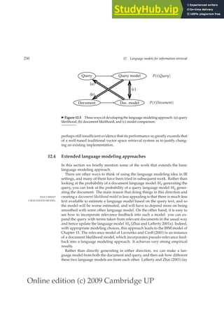


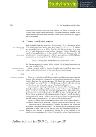
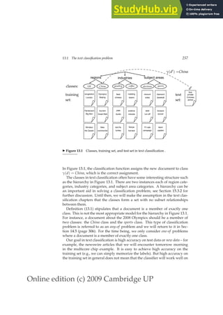

![Online edition (c) 2009 Cambridge UP
13.2 Naive Bayes text classification 259
actually done in most implementations of NB is:
cmap = arg max
c∈C
[log P̂(c) + ∑
1≤k≤nd
log P̂(tk|c)].
(13.4)
Equation (13.4) has a simple interpretation. Each conditional parameter
log P̂(tk|c) is a weight that indicates how good an indicator tk is for c. Sim-
ilarly, the prior log P̂(c) is a weight that indicates the relative frequency of
c. More frequent classes are more likely to be the correct class than infre-
quent classes. The sum of log prior and term weights is then a measure of
how much evidence there is for the document being in the class, and Equa-
tion (13.4) selects the class for which we have the most evidence.
We will initially work with this intuitive interpretation of the multinomial
NB model and defer a formal derivation to Section 13.4.
How do we estimate the parameters P̂(c) and P̂(tk|c)? We first try the
maximum likelihood estimate (MLE; Section 11.3.2, page 226), which is sim-
ply the relative frequency and corresponds to the most likely value of each
parameter given the training data. For the priors this estimate is:
P̂(c) =
Nc
N
,
(13.5)
where Nc is the number of documents in class c and N is the total number of
documents.
We estimate the conditional probability P̂(t|c) as the relative frequency of
term t in documents belonging to class c:
P̂(t|c) =
Tct
∑t′∈V Tct′
,
(13.6)
where Tct is the number of occurrences of t in training documents from class
c, including multiple occurrences of a term in a document. We have made the
positional independence assumption here, which we will discuss in more detail
in the next section: Tct is a count of occurrences in all positions k in the doc-
uments in the training set. Thus, we do not compute different estimates for
different positions and, for example, if a word occurs twice in a document,
in positions k1 and k2, then P̂(tk1
|c) = P̂(tk2
|c).
The problem with the MLE estimate is that it is zero for a term–class combi-
nation that did not occur in the training data. If the term WTO in the training
data only occurred in China documents, then the MLE estimates for the other
classes, for example UK, will be zero:
P̂(WTO|UK) = 0.
Now, the one-sentence document Britain is a member of the WTO will get a
conditional probability of zero for UK because we are multiplying the condi-
tional probabilities for all terms in Equation (13.2). Clearly, the model should](https://image.slidesharecdn.com/anintroductiontoinformationretrieval-230807170822-1d67eee0/85/An-Introduction-to-Information-Retrieval-pdf-284-320.jpg)
![Online edition (c) 2009 Cambridge UP
260 13 Text classification and Naive Bayes
TRAINMULTINOMIALNB(C, D)
1 V ← EXTRACTVOCABULARY(D)
2 N ← COUNTDOCS(D)
3 for each c ∈ C
4 do Nc ← COUNTDOCSINCLASS(D, c)
5 prior[c] ← Nc/N
6 textc ← CONCATENATETEXTOFALLDOCSINCLASS(D, c)
7 for each t ∈ V
8 do Tct ← COUNTTOKENSOFTERM(textc, t)
9 for each t ∈ V
10 do condprob[t][c] ← Tct+1
∑t′ (Tct′+1)
11 return V, prior, condprob
APPLYMULTINOMIALNB(C, V, prior, condprob, d)
1 W ← EXTRACTTOKENSFROMDOC(V, d)
2 for each c ∈ C
3 do score[c] ← log prior[c]
4 for each t ∈ W
5 do score[c] += log condprob[t][c]
6 return arg maxc∈C score[c]
◮ Figure 13.2 Naive Bayes algorithm (multinomial model): Training and testing.
assign a high probability to the UK class because the term Britain occurs. The
problem is that the zero probability for WTO cannot be “conditioned away,”
no matter how strong the evidence for the class UK from other features. The
estimate is 0 because of sparseness: The training data are never large enough
SPARSENESS
to represent the frequency of rare events adequately, for example, the fre-
quency of WTO occurring in UK documents.
To eliminate zeros, we use add-one or Laplace smoothing, which simply adds
ADD-ONE SMOOTHING
one to each count (cf. Section 11.3.2):
P̂(t|c) =
Tct + 1
∑t′∈V(Tct′ + 1)
=
Tct + 1
(∑t′∈V Tct′) + B
,
(13.7)
where B = |V| is the number of terms in the vocabulary. Add-one smoothing
can be interpreted as a uniform prior (each term occurs once for each class)
that is then updated as evidence from the training data comes in. Note that
this is a prior probability for the occurrence of a term as opposed to the prior
probability of a class which we estimate in Equation (13.5) on the document
level.](https://image.slidesharecdn.com/anintroductiontoinformationretrieval-230807170822-1d67eee0/85/An-Introduction-to-Information-Retrieval-pdf-285-320.jpg)

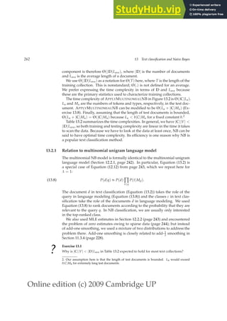
![Online edition (c) 2009 Cambridge UP
13.3 The Bernoulli model 263
TRAINBERNOULLINB(C, D)
1 V ← EXTRACTVOCABULARY(D)
2 N ← COUNTDOCS(D)
3 for each c ∈ C
4 do Nc ← COUNTDOCSINCLASS(D, c)
5 prior[c] ← Nc/N
6 for each t ∈ V
7 do Nct ← COUNTDOCSINCLASSCONTAININGTERM(D, c, t)
8 condprob[t][c] ← (Nct + 1)/(Nc + 2)
9 return V, prior, condprob
APPLYBERNOULLINB(C, V, prior, condprob, d)
1 Vd ← EXTRACTTERMSFROMDOC(V, d)
2 for each c ∈ C
3 do score[c] ← log prior[c]
4 for each t ∈ V
5 do if t ∈ Vd
6 then score[c] += log condprob[t][c]
7 else score[c] += log(1 − condprob[t][c])
8 return arg maxc∈C score[c]
◮ Figure 13.3 NB algorithm (Bernoulli model): Training and testing. The add-one
smoothing in Line 8 (top) is in analogy to Equation (13.7) with B = 2.
13.3 The Bernoulli model
There are two different ways we can set up an NB classifier. The model we in-
troduced in the previous section is the multinomial model. It generates one
term from the vocabulary in each position of the document, where we as-
sume a generative model that will be discussed in more detail in Section 13.4
(see also page 237).
An alternative to the multinomial model is the multivariate Bernoulli model
or Bernoulli model. It is equivalent to the binary independence model of Sec-
BERNOULLI MODEL
tion 11.3 (page 222), which generates an indicator for each term of the vo-
cabulary, either 1 indicating presence of the term in the document or 0 indi-
cating absence. Figure 13.3 presents training and testing algorithms for the
Bernoulli model. The Bernoulli model has the same time complexity as the
multinomial model.
The different generation models imply different estimation strategies and
different classification rules. The Bernoulli model estimates P̂(t|c) as the frac-
tion of documents of class c that contain term t (Figure 13.3, TRAINBERNOULLI-](https://image.slidesharecdn.com/anintroductiontoinformationretrieval-230807170822-1d67eee0/85/An-Introduction-to-Information-Retrieval-pdf-288-320.jpg)


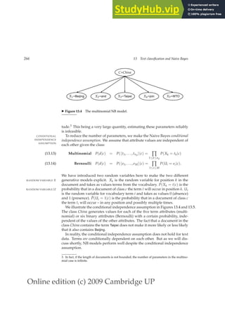

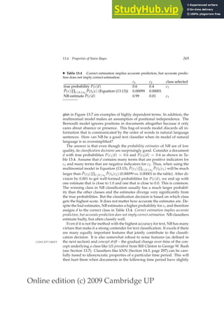

![Online edition (c) 2009 Cambridge UP
13.5 Feature selection 271
SELECTFEATURES(D, c, k)
1 V ← EXTRACTVOCABULARY(D)
2 L ← []
3 for each t ∈ V
4 do A(t, c) ← COMPUTEFEATUREUTILITY(D, t, c)
5 APPEND(L, hA(t, c), ti)
6 return FEATURESWITHLARGESTVALUES(L, k)
◮ Figure 13.6 Basic feature selection algorithm for selecting the k best features.
?
Exercise 13.2 [⋆]
Which of the documents in Table 13.5 have identical and different bag of words rep-
resentations for (i) the Bernoulli model (ii) the multinomial model? If there are differ-
ences, describe them.
Exercise 13.3
The rationale for the positional independence assumption is that there is no useful
information in the fact that a term occurs in position k of a document. Find exceptions.
Consider formulaic documents with a fixed document structure.
Exercise 13.4
Table 13.3 gives Bernoulli and multinomial estimates for the word the. Explain the
difference.
13.5 Feature selection
Feature selection is the process of selecting a subset of the terms occurring
FEATURE SELECTION
in the training set and using only this subset as features in text classifica-
tion. Feature selection serves two main purposes. First, it makes training
and applying a classifier more efficient by decreasing the size of the effective
vocabulary. This is of particular importance for classifiers that, unlike NB,
are expensive to train. Second, feature selection often increases classifica-
tion accuracy by eliminating noise features. A noise feature is one that, when
NOISE FEATURE
added to the document representation, increases the classification error on
new data. Suppose a rare term, say arachnocentric, has no information about
a class, say China, but all instances of arachnocentric happen to occur in China
documents in our training set. Then the learning method might produce a
classifier that misassigns test documents containing arachnocentric to China.
Such an incorrect generalization from an accidental property of the training
set is called overfitting.
OVERFITTING
We can view feature selection as a method for replacing a complex clas-
sifier (using all features) with a simpler one (using a subset of the features).](https://image.slidesharecdn.com/anintroductiontoinformationretrieval-230807170822-1d67eee0/85/An-Introduction-to-Information-Retrieval-pdf-296-320.jpg)
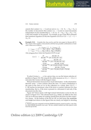
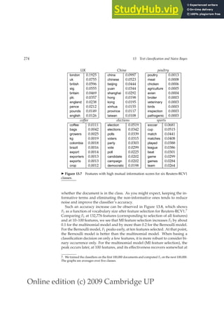
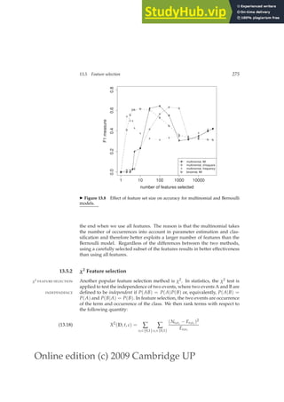

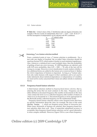
![Online edition (c) 2009 Cambridge UP
13.6 Evaluation of text classification 279
Peak effectiveness is virtually the same for both methods. χ2 reaches this
peak later, at 300 features, probably because the rare, but highly significant
features it selects initially do not cover all documents in the class. However,
features selected later (in the range of 100–300)are of better quality than those
selected by MI.
All three methods – MI, χ2 and frequency based – are greedy methods.
GREEDY FEATURE
SELECTION They may select features that contribute no incremental information over
previously selected features. In Figure 13.7, kong is selected as the seventh
term even though it is highly correlated with previously selected hong and
therefore redundant. Although such redundancy can negatively impact ac-
curacy, non-greedy methods (see Section 13.7 for references) are rarely used
in text classification due to their computational cost.
?
Exercise 13.5
Consider the following frequencies for the class coffee for four terms in the first 100,000
documents of Reuters-RCV1:
term N00 N01 N10 N11
brazil 98,012 102 1835 51
council 96,322 133 3525 20
producers 98,524 119 1118 34
roasted 99,824 143 23 10
Select two of these four terms based on (i) χ2, (ii) mutual information, (iii) frequency.
13.6 Evaluation of text classification
] Historically, the classic Reuters-21578 collection was the main benchmark
for text classification evaluation. This is a collection of 21,578 newswire ar-
ticles, originally collected and labeled by Carnegie Group, Inc. and Reuters,
Ltd. in the course of developing the CONSTRUE text classification system.
It is much smaller than and predates the Reuters-RCV1 collection discussed
in Chapter 4 (page 69). The articles are assigned classes from a set of 118
topic categories. A document may be assigned several classes or none, but
the commonest case is single assignment (documents with at least one class
received an average of 1.24 classes). The standard approach to this any-of
problem (Chapter 14, page 306) is to learn 118 two-class classifiers, one for
each class, where the two-class classifier for class c is the classifier for the two
TWO-CLASS CLASSIFIER
classes c and its complement c.
For each of these classifiers, we can measure recall, precision, and accu-
racy. In recent work, people almost invariably use the ModApte split, which
MODAPTE SPLIT
includes only documents that were viewed and assessed by a human indexer,](https://image.slidesharecdn.com/anintroductiontoinformationretrieval-230807170822-1d67eee0/85/An-Introduction-to-Information-Retrieval-pdf-304-320.jpg)
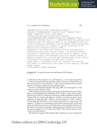
![Online edition (c) 2009 Cambridge UP
282 13 Text classification and Naive Bayes
◮ Table 13.8 Macro- and microaveraging. “Truth” is the true class and “call” the
decision of the classifier. In this example, macroaveraged precision is [10/(10 + 10) +
90/(10 + 90)]/2 = (0.5 + 0.9)/2 = 0.7. Microaveraged precision is 100/(100 + 20) ≈
0.83.
class 1
truth: truth:
yes no
call:
yes
10 10
call:
no
10 970
class 2
truth: truth:
yes no
call:
yes
90 10
call:
no
10 890
pooled table
truth: truth:
yes no
call:
yes
100 20
call:
no
20 1860
◮ Table 13.9 Text classification effectiveness numbers on Reuters-21578 for F1 (in
percent). Results from Li and Yang (2003) (a), Joachims (1998) (b: kNN) and Dumais
et al. (1998) (b: NB, Rocchio, trees, SVM).
(a) NB Rocchio kNN SVM
micro-avg-L (90 classes) 80 85 86 89
macro-avg (90 classes) 47 59 60 60
(b) NB Rocchio kNN trees SVM
earn 96 93 97 98 98
acq 88 65 92 90 94
money-fx 57 47 78 66 75
grain 79 68 82 85 95
crude 80 70 86 85 89
trade 64 65 77 73 76
interest 65 63 74 67 78
ship 85 49 79 74 86
wheat 70 69 77 93 92
corn 65 48 78 92 90
micro-avg (top 10) 82 65 82 88 92
micro-avg-D (118 classes) 75 62 n/a n/a 87
Rocchio and kNN. In addition, we give numbers for decision trees, an impor-
DECISION TREES
tant classification method we do not cover. The bottom part of the table
shows that there is considerable variation from class to class. For instance,
NB beats kNN on ship, but is much worse on money-fx.
Comparing parts (a) and (b) of the table, one is struck by the degree to
which the cited papers’ results differ. This is partly due to the fact that the
numbers in (b) are break-even scores (cf. page 161) averaged over 118 classes,
whereas the numbers in (a) are true F1 scores (computed without any know-](https://image.slidesharecdn.com/anintroductiontoinformationretrieval-230807170822-1d67eee0/85/An-Introduction-to-Information-Retrieval-pdf-307-320.jpg)

![Online edition (c) 2009 Cambridge UP
284 13 Text classification and Naive Bayes
◮ Table 13.10 Data for parameter estimation exercise.
docID words in document in c = China?
training set 1 Taipei Taiwan yes
2 Macao Taiwan Shanghai yes
3 Japan Sapporo no
4 Sapporo Osaka Taiwan no
test set 5 Taiwan Taiwan Sapporo ?
tion about the test set was used in developing the classifier, the results of this
experiment should be indicative of actual performance in practice.
This ideal often cannot be met; researchers tend to evaluate several sys-
tems on the same test set over a period of several years. But it is neverthe-
less highly important to not look at the test data and to run systems on it as
sparingly as possible. Beginners often violate this rule, and their results lose
validity because they have implicitly tuned their system to the test data sim-
ply by running many variant systems and keeping the tweaks to the system
that worked best on the test set.
?
Exercise 13.6 [⋆⋆]
Assume a situation where every document in the test collection has been assigned
exactly one class, and that a classifier also assigns exactly one class to each document.
This setup is called one-of classification (Section 14.5, page 306). Show that in one-of
classification (i) the total number of false positive decisions equals the total number
of false negative decisions and (ii) microaveraged F1 and accuracy are identical.
Exercise 13.7
The class priors in Figure 13.2 are computed as the fraction of documents in the class
as opposed to the fraction of tokens in the class. Why?
Exercise 13.8
The function APPLYMULTINOMIALNB in Figure 13.2 has time complexity Θ(La +
|C|La). How would you modify the function so that its time complexity is Θ(La +
|C|Ma)?
Exercise 13.9
Based on the data in Table 13.10, (i) estimate a multinomial Naive Bayes classifier, (ii)
apply the classifier to the test document, (iii) estimate a Bernoulli NB classifier, (iv)
apply the classifier to the test document. You need not estimate parameters that you
don’t need for classifying the test document.
Exercise 13.10
Your task is to classify words as English or not English. Words are generated by a
source with the following distribution:](https://image.slidesharecdn.com/anintroductiontoinformationretrieval-230807170822-1d67eee0/85/An-Introduction-to-Information-Retrieval-pdf-309-320.jpg)


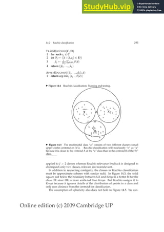
![Online edition (c) 2009 Cambridge UP
296 14 Vector space classification
mode time complexity
training Θ(|D|Lave + |C||V|)
testing Θ(La + |C|Ma) = Θ(|C|Ma)
◮ Table 14.2 Training and test times for Rocchio classification. Lave is the average
number of tokens per document. La and Ma are the numbers of tokens and types,
respectively, in the test document. Computing Euclidean distance between the class
centroids and a document is Θ(|C|Ma).
not represent the “a” class well with a single prototype because it has two
clusters. Rocchio often misclassifies this type of multimodal class. A text clas-
MULTIMODAL CLASS
sification example for multimodality is a country like Burma, which changed
its name to Myanmar in 1989. The two clusters before and after the name
change need not be close to each other in space. We also encountered the
problem of multimodality in relevance feedback (Section 9.1.2, page 184).
Two-class classification is another case where classes are rarely distributed
like spheres with similar radii. Most two-class classifiers distinguish between
a class like China that occupies a small region of the space and its widely
scattered complement. Assuming equal radii will result in a large number
of false positives. Most two-class classification problems therefore require a
modified decision rule of the form:
Assign d to class c iff |~
µ(c) −~
v(d)| |~
µ(c) −~
v(d)| − b
for a positive constant b. As in Rocchio relevance feedback, the centroid of
the negative documents is often not used at all, so that the decision criterion
simplifies to |~
µ(c) −~
v(d)| b′ for a positive constant b′.
Table 14.2 gives the time complexity of Rocchio classification.2 Adding all
documents to their respective (unnormalized) centroid is Θ(|D|Lave) (as op-
posed to Θ(|D||V|)) since we need only consider non-zero entries. Dividing
each vector sum by the size of its class to compute the centroid is Θ(|V|).
Overall, training time is linear in the size of the collection (cf. Exercise 13.1).
Thus, Rocchio classification and Naive Bayes have the same linear training
time complexity.
In the next section, we will introduce another vector space classification
method, kNN, that deals better with classes that have non-spherical, discon-
nected or other irregular shapes.
? Exercise 14.2 [⋆]
Show that Rocchio classification can assign a label to a document that is different from
its training set label.
2. We write Θ(|D|Lave) for Θ(T) and assume that the length of test documents is bounded as
we did on page 262.](https://image.slidesharecdn.com/anintroductiontoinformationretrieval-230807170822-1d67eee0/85/An-Introduction-to-Information-Retrieval-pdf-321-320.jpg)

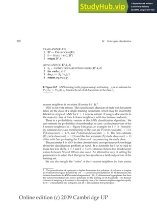
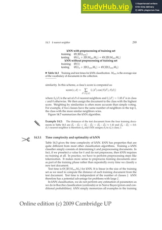

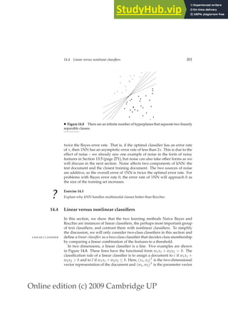

![Online edition (c) 2009 Cambridge UP
14.4 Linear versus nonlinear classifiers 303
ti wi d1i d2i ti wi d1i d2i
prime 0.70 0 1 dlrs -0.71 1 1
rate 0.67 1 0 world -0.35 1 0
interest 0.63 0 0 sees -0.33 0 0
rates 0.60 0 0 year -0.25 0 0
discount 0.46 1 0 group -0.24 0 0
bundesbank 0.43 0 0 dlr -0.24 0 0
◮ Table 14.4 A linear classifier. The dimensions ti and parameters wi of a linear
classifier for the class interest (as in interest rate) in Reuters-21578. The threshold is
b = 0. Terms like dlr and world have negative weights because they are indicators for
the competing class currency.
We choose class c if the odds are greater than 1 or, equivalently, if the log
odds are greater than 0. It is easy to see that Equation (14.5) is an instance
of Equation (14.3) for wi = log[P̂(ti|c)/P̂(ti|c̄)], xi = number of occurrences
of ti in d, and b = − log[P̂(c)/P̂(c̄)]. Here, the index i, 1 ≤ i ≤ M, refers
to terms of the vocabulary (not to positions in d as k does; cf. Section 13.4.1,
page 270) and ~
x and ~
w are M-dimensional vectors. So in log space, Naive
Bayes is a linear classifier.
✎ Example 14.3: Table 14.4 defines a linear classifier for the category interest in
Reuters-21578 (see Section 13.6, page 279). We assign document ~
d1 “rate discount
dlrs world” to interest since ~
wT~
d1 = 0.67 · 1 + 0.46 · 1 + (−0.71) · 1 + (−0.35) · 1 =
0.07 0 = b. We assign ~
d2 “prime dlrs” to the complement class (not in interest) since
~
wT~
d2 = −0.01 ≤ b. For simplicity, we assume a simple binary vector representation
in this example: 1 for occurring terms, 0 for non-occurring terms.
Figure 14.10 is a graphical example of a linear problem, which we define to
mean that the underlying distributions P(d|c) and P(d|c) of the two classes
are separated by a line. We call this separating line the class boundary. It is
CLASS BOUNDARY
the “true” boundary of the two classes and we distinguish it from the deci-
sion boundary that the learning method computes to approximate the class
boundary.
As is typical in text classification, there are some noise documents in Fig-
NOISE DOCUMENT
ure 14.10 (marked with arrows) that do not fit well into the overall distri-
bution of the classes. In Section 13.5 (page 271), we defined a noise feature
as a misleading feature that, when included in the document representation,
on average increases the classification error. Analogously, a noise document
is a document that, when included in the training set, misleads the learn-
ing method and increases classification error. Intuitively, the underlying
distribution partitions the representation space into areas with mostly ho-](https://image.slidesharecdn.com/anintroductiontoinformationretrieval-230807170822-1d67eee0/85/An-Introduction-to-Information-Retrieval-pdf-328-320.jpg)

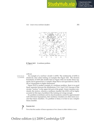


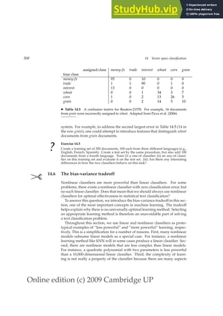
![Online edition (c) 2009 Cambridge UP
14.6 The bias-variance tradeoff 309
of learning (such as feature selection, cf. (Section 13.5, page 271), regulariza-
tion, and constraints such as margin maximization in Chapter 15) that make
a learning method either more powerful or less powerful without affecting
the type of classifier that is the final result of learning – regardless of whether
that classifier is linear or nonlinear. We refer the reader to the publications
listed in Section 14.7 for a treatment of the bias-variance tradeoff that takes
into account these complexities. In this section, linear and nonlinear classi-
fiers will simply serve as proxies for weaker and stronger learning methods
in text classification.
We first need to state our objective in text classification more precisely. In
Section 13.1 (page 256), we said that we want to minimize classification er-
ror on the test set. The implicit assumption was that training documents
and test documents are generated according to the same underlying distri-
bution. We will denote this distribution P(hd, ci) where d is the document
and c its label or class. Figures 13.4 and 13.5 were examples of generative
models that decompose P(hd, ci) into the product of P(c) and P(d|c). Fig-
ures 14.10 and 14.11 depict generative models for hd, ci with d ∈ R2 and
c ∈ {square, solid circle}.
In this section, instead of using the number of correctly classified test doc-
uments (or, equivalently, the error rate on test documents) as evaluation
measure, we adopt an evaluation measure that addresses the inherent un-
certainty of labeling. In many text classification problems, a given document
representation can arise from documents belonging to different classes. This
is because documents from different classes can be mapped to the same doc-
ument representation. For example, the one-sentence documents China sues
France and France sues China are mapped to the same document representa-
tion d′ = {China, France, sues} in a bag of words model. But only the latter
document is relevant to the class c′ = legal actions brought by France (which
might be defined, for example, as a standing query by an international trade
lawyer).
To simplify the calculations in this section, we do not count the number
of errors on the test set when evaluating a classifier, but instead look at how
well the classifier estimates the conditional probability P(c|d) of a document
being in a class. In the above example, we might have P(c′|d′) = 0.5.
Our goal in text classification then is to find a classifier γ such that, aver-
aged over documents d, γ(d) is as close as possible to the true probability
P(c|d). We measure this using mean squared error:
MSE(γ) = Ed[γ(d) − P(c|d)]2
(14.6)
where Ed is the expectation with respect to P(d). The mean squared error
term gives partial credit for decisions by γ that are close if not completely
right.](https://image.slidesharecdn.com/anintroductiontoinformationretrieval-230807170822-1d67eee0/85/An-Introduction-to-Information-Retrieval-pdf-334-320.jpg)
![Online edition (c) 2009 Cambridge UP
310 14 Vector space classification
E[x − α]2
= Ex2
− 2Exα + α2
(14.8)
= (Ex)2
− 2Exα + α2
+Ex2
− 2(Ex)2
+ (Ex)2
= [Ex − α]2
+Ex2
− E2x(Ex) + E(Ex)2
= [Ex − α]2
+ E[x − Ex]2
EDEd[ΓD(d) − P(c|d)]2
= EdED[ΓD(d) − P(c|d)]2
(14.9)
= Ed[ [EDΓD(d) − P(c|d)]2
+ED[ΓD(d) − EDΓD(d)]2
]
◮ Figure 14.13 Arithmetic transformations for the bias-variance decomposition.
For the derivation of Equation (14.9), we set α = P(c|d) and x = ΓD(d) in Equa-
tion (14.8).
We define a classifier γ to be optimal for a distribution P(hd, ci) if it mini-
OPTIMAL CLASSIFIER
mizes MSE(γ).
Minimizing MSE is a desideratum for classifiers. We also need a criterion
for learning methods. Recall that we defined a learning method Γ as a function
that takes a labeled training set D as input and returns a classifier γ.
For learning methods, we adopt as our goal to find a Γ that, averaged over
training sets, learns classifiers γ with minimal MSE. We can formalize this as
minimizing learning error:
LEARNING ERROR
learning-error(Γ) = ED[MSE(Γ(D))]
(14.7)
where ED is the expectation over labeled training sets. To keep things simple,
we can assume that training sets have a fixed size – the distribution P(hd, ci)
then defines a distribution P(D) over training sets.
We can use learning error as a criterion for selecting a learning method in
statistical text classification. A learning method Γ is optimal for a distribution
OPTIMAL LEARNING
METHOD P(D) if it minimizes the learning error.
Writing ΓD for Γ(D) for better readability, we can transform Equation (14.7)
as follows:
learning-error(Γ) = ED[MSE(ΓD)]
= EDEd[ΓD(d) − P(c|d)]2
(14.10)
= Ed[bias(Γ, d) + variance(Γ, d)]
(14.11)](https://image.slidesharecdn.com/anintroductiontoinformationretrieval-230807170822-1d67eee0/85/An-Introduction-to-Information-Retrieval-pdf-335-320.jpg)
![Online edition (c) 2009 Cambridge UP
14.6 The bias-variance tradeoff 311
bias(Γ, d) = [P(c|d) − EDΓD(d)]2
(14.12)
variance(Γ, d) = ED[ΓD(d) − EDΓD(d)]2
(14.13)
where the equivalence between Equations (14.10) and (14.11) is shown in
Equation (14.9) in Figure 14.13. Note that d and D are independent of each
other. In general, for a random document d and a random training set D, D
does not contain a labeled instance of d.
Bias is the squared difference between P(c|d), the true conditional prob-
BIAS
ability of d being in c, and ΓD(d), the prediction of the learned classifier,
averaged over training sets. Bias is large if the learning method produces
classifiers that are consistently wrong. Bias is small if (i) the classifiers are
consistently right or (ii) different training sets cause errors on different docu-
ments or (iii) different training sets cause positive and negative errors on the
same documents, but that average out to close to 0. If one of these three con-
ditions holds, then EDΓD(d), the expectation over all training sets, is close to
P(c|d).
Linear methods like Rocchio and Naive Bayes have a high bias for non-
linear problems because they can only model one type of class boundary, a
linear hyperplane. If the generative model P(hd, ci) has a complex nonlinear
class boundary, the bias term in Equation (14.11) will be high because a large
number of points will be consistently misclassified. For example, the circular
enclave in Figure 14.11 does not fit a linear model and will be misclassified
consistently by linear classifiers.
We can think of bias as resulting from our domain knowledge (or lack
thereof) that we build into the classifier. If we know that the true boundary
between the two classes is linear, then a learning method that produces linear
classifiers is more likely to succeed than a nonlinear method. But if the true
class boundary is not linear and we incorrectly bias the classifier to be linear,
then classification accuracy will be low on average.
Nonlinear methods like kNN have low bias. We can see in Figure 14.6 that
the decision boundaries of kNN are variable – depending on the distribu-
tion of documents in the training set, learned decision boundaries can vary
greatly. As a result, each document has a chance of being classified correctly
for some training sets. The average prediction EDΓD(d) is therefore closer to
P(c|d) and bias is smaller than for a linear learning method.
Variance is the variation of the prediction of learned classifiers: the aver-
VARIANCE
age squared difference between ΓD(d) and its average EDΓD(d). Variance is
large if different training sets D give rise to very different classifiers ΓD. It is
small if the training set has a minor effect on the classification decisions ΓD
makes, be they correct or incorrect. Variance measures how inconsistent the
decisions are, not whether they are correct or incorrect.
Linear learning methods have low variance because most randomly drawn
training sets produce similar decision hyperplanes. The decision lines pro-](https://image.slidesharecdn.com/anintroductiontoinformationretrieval-230807170822-1d67eee0/85/An-Introduction-to-Information-Retrieval-pdf-336-320.jpg)
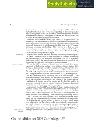
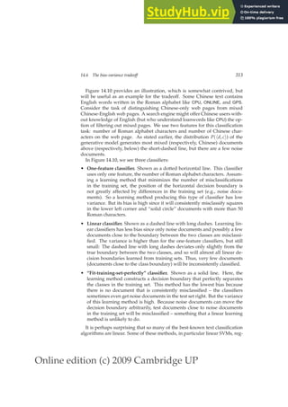
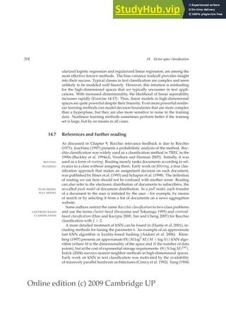
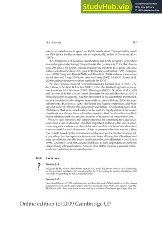
![Online edition (c) 2009 Cambridge UP
316 14 Vector space classification
0 1 2 3 4 5 6 7 8
0
1
2
3
4
5
6
7
8
a
x
b
c
◮ Figure 14.14 Example for differences between Euclidean distance, dot product
similarity and cosine similarity. The vectors are ~
a = (0.5 1.5)T, ~
x = (2 2)T, ~
b =
(4 4)T, and~
c = (8 6)T.
plement Rocchio classification and kNN classification, for example, the Bow toolkit
(McCallum 1996).
Exercise 14.8
Download 20 Newgroups (page 154) and train and test Rocchio and kNN classifiers
for its 20 classes.
Exercise 14.9
Show that the decision boundaries in Rocchio classification are, as in kNN, given by
the Voronoi tessellation.
Exercise 14.10 [⋆]
Computing the distance between a dense centroid and a sparse vector is Θ(M) for
a naive implementation that iterates over all M dimensions. Based on the equality
∑(xi − µi)2 = 1.0 + ∑ µ2
i − 2 ∑ xiµi and assuming that ∑ µ2
i has been precomputed,
write down an algorithm that is Θ(Ma) instead, where Ma is the number of distinct
terms in the test document.
Exercise 14.11 [⋆ ⋆ ⋆]
Prove that the region of the plane consisting of all points with the same k nearest
neighbors is a convex polygon.
Exercise 14.12
Design an algorithm that performs an efficient 1NN search in 1 dimension (where
efficiency is with respect to the number of documents N). What is the time complexity
of the algorithm?
Exercise 14.13 [⋆ ⋆ ⋆]
Design an algorithm that performs an efficient 1NN search in 2 dimensions with at
most polynomial (in N) preprocessing time.](https://image.slidesharecdn.com/anintroductiontoinformationretrieval-230807170822-1d67eee0/85/An-Introduction-to-Information-Retrieval-pdf-341-320.jpg)
![Online edition (c) 2009 Cambridge UP
14.8 Exercises 317
b
b
◮ Figure 14.15 A simple non-separable set of points.
Exercise 14.14 [⋆ ⋆ ⋆]
Can one design an exact efficient algorithm for 1NN for very large M along the ideas
you used to solve the last exercise?
Exercise 14.15
Show that Equation (14.4) defines a hyperplane with ~
w = ~
µ(c1) − ~
µ(c2) and b =
0.5 ∗ (|~
µ(c1)|2 − |~
µ(c2)|2).
Exercise 14.16
We can easily construct non-separable data sets in high dimensions by embedding
a non-separable set like the one shown in Figure 14.15. Consider embedding Fig-
ure 14.15 in 3D and then perturbing the 4 points slightly (i.e., moving them a small
distance in a random direction). Why would you expect the resulting configuration
to be linearly separable? How likely is then a non-separable set of m ≪ M points in
M-dimensional space?
Exercise 14.17
Assuming two classes, show that the percentage of non-separable assignments of the
vertices of a hypercube decreases with dimensionality M for M 1. For example,
for M = 1 the proportion of non-separable assignments is 0, for M = 2, it is 2/16.
One of the two non-separable cases for M = 2 is shown in Figure 14.15, the other is
its mirror image. Solve the exercise either analytically or by simulation.
Exercise 14.18
Although we point out the similarities of Naive Bayes with linear vector space classi-
fiers, it does not make sense to represent count vectors (the document representations
in NB) in a continuous vector space. There is however a formalization of NB that is
analogous to Rocchio. Show that NB assigns a document to the class (represented as
a parameter vector) whose Kullback-Leibler (KL) divergence (Section 12.4, page 251)
to the document (represented as a count vector as in Section 13.4.1 (page 270), nor-
malized to sum to 1) is smallest.](https://image.slidesharecdn.com/anintroductiontoinformationretrieval-230807170822-1d67eee0/85/An-Introduction-to-Information-Retrieval-pdf-342-320.jpg)


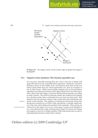
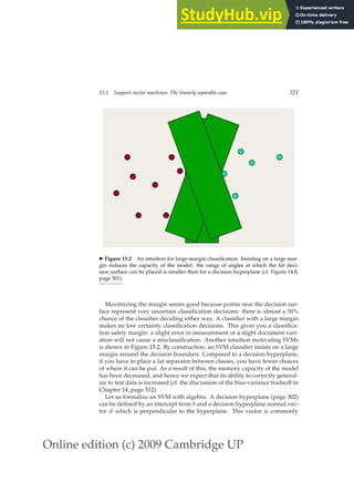

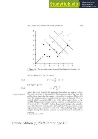
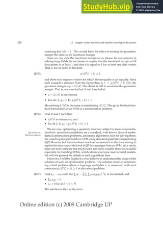
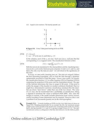
![Online edition (c) 2009 Cambridge UP
326 15 Support vector machines and machine learning on documents
Therefore, it passes through (1.5, 2). So, the SVM decision boundary is:
y = x1 + 2x2 − 5.5
Working algebraically, with the standard constraint that sign(yi(~
wT~
xi + b)) ≥ 1,
we seek to minimize |~
w|. This happens when this constraint is satisfied with equality
by the two support vectors. Further we know that the solution is ~
w = (a, 2a) for some
a. So we have that:
a + 2a + b = −1
2a + 6a + b = 1
Therefore, a = 2/5 and b = −11/5. So the optimal hyperplane is given by ~
w =
(2/5, 4/5) and b = −11/5.
The margin ρ is 2/|~
w| = 2/
√
4/25 + 16/25 = 2/(2
√
5/5) =
√
5. This answer can
be confirmed geometrically by examining Figure 15.4.
?
Exercise 15.1 [⋆]
What is the minimum number of support vectors that there can be for a data set
(which contains instances of each class)?
Exercise 15.2 [⋆⋆]
The basis of being able to use kernels in SVMs (see Section 15.2.3) is that the classifica-
tion function can be written in the form of Equation (15.9) (where, for large problems,
most αi are 0). Show explicitly how the classification function could be written in this
form for the data set from Example 15.1. That is, write f as a function where the data
points appear and the only variable is ~
x.
Exercise 15.3 [⋆⋆]
Install an SVM package such as SVMlight (http://svmlight.joachims.org/), and build an
SVM for the data set discussed in Example 15.1. Confirm that the program gives the
same solution as the text. For SVMlight, or another package that accepts the same
training data format, the training file would be:
+1 1:2 2:3
−1 1:2 2:0
−1 1:1 2:1
The training command for SVMlight is then:
svm_learn -c 1 -a alphas.dat train.dat model.dat
The -c 1 option is needed to turn off use of the slack variables that we discuss in
Section 15.2.1. Check that the norm of the weight vector agrees with what we found
in Example 15.1. Examine the file alphas.dat which contains the αi values, and check
that they agree with your answers in Exercise 15.2.](https://image.slidesharecdn.com/anintroductiontoinformationretrieval-230807170822-1d67eee0/85/An-Introduction-to-Information-Retrieval-pdf-351-320.jpg)

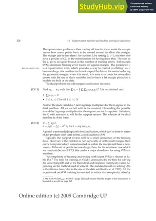
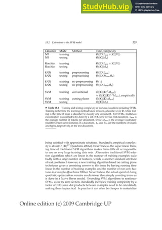

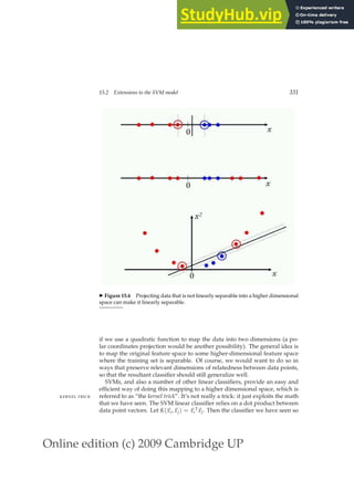
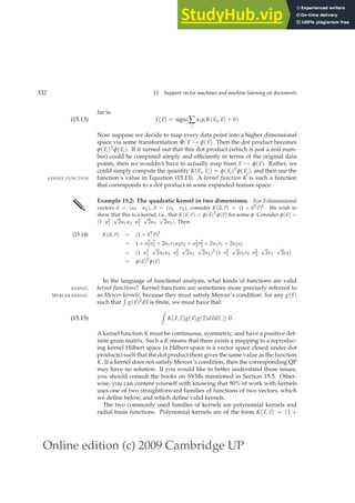


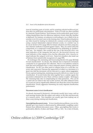

![Online edition (c) 2009 Cambridge UP
15.4 Machine learning methods in ad hoc information retrieval 341
presumably works because most such sentences are somehow more central
to the concerns of the document.
?
Exercise 15.4 [⋆⋆]
Spam email often makes use of various cloaking techniques to try to get through. One
method is to pad or substitute characters so as to defeat word-based text classifiers.
For example, you see terms like the following in spam email:
Rep1icaRolex bonmus Viiiaaaagra pi11z
PHARlbdMACY [LEV]i[IT]l[RA] se∧xual ClAfLlS
Discuss how you could engineer features that would largely defeat this strategy.
Exercise 15.5 [⋆⋆]
Another strategy often used by purveyors of email spam is to follow the message
they wish to send (such as buying a cheap stock or whatever) with a paragraph of
text from another innocuous source (such as a news article). Why might this strategy
be effective? How might it be addressed by a text classifier?
Exercise 15.6 [⋆]
What other kinds of features appear as if they would be useful in an email spam
classifier?
15.4 Machine learning methods in ad hoc information retrieval
Rather than coming up with term and document weighting functions by
hand, as we primarily did in Chapter 6, we can view different sources of rele-
vance signal (cosine score, title match, etc.) as features in a learning problem.
A classifier that has been fed examples of relevant and nonrelevant docu-
ments for each of a set of queries can then figure out the relative weights
of these signals. If we configure the problem so that there are pairs of a
document and a query which are assigned a relevance judgment of relevant
or nonrelevant, then we can think of this problem too as a text classification
problem. Taking such a classification approach is not necessarily best, and
we present an alternative in Section 15.4.2. Nevertheless, given the material
we have covered, the simplest place to start is to approach this problem as
a classification problem, by ordering the documents according to the confi-
dence of a two-class classifier in its relevance decision. And this move is not
purely pedagogical; exactly this approach is sometimes used in practice.
15.4.1 A simple example of machine-learned scoring
In this section we generalize the methodology of Section 6.1.2 (page 113) to
machine learning of the scoring function. In Section 6.1.2 we considered a
case where we had to combine Boolean indicators of relevance; here we con-
sider more general factors to further develop the notion of machine-learned](https://image.slidesharecdn.com/anintroductiontoinformationretrieval-230807170822-1d67eee0/85/An-Introduction-to-Information-Retrieval-pdf-366-320.jpg)
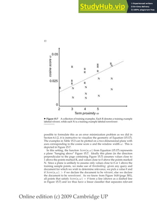

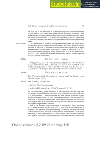
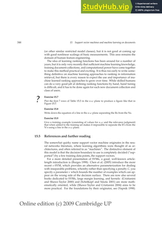
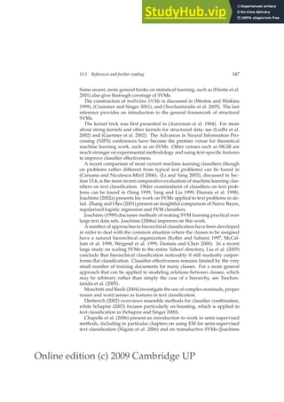

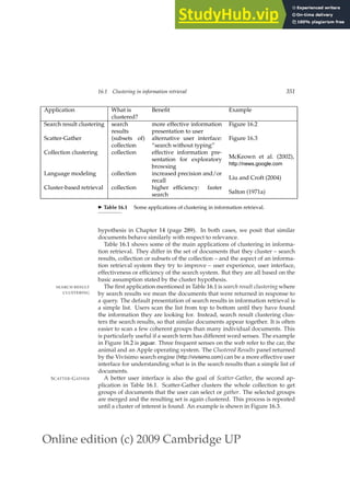
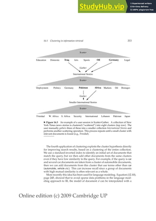
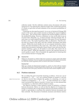
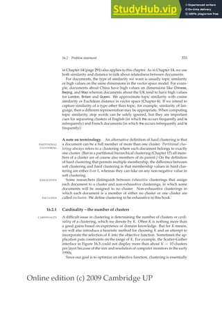


![Online edition (c) 2009 Cambridge UP
358 16 Flat clustering
mation or NMI:
NMI(Ω, C) =
I(Ω; C)
[H(Ω) + H(C)]/2
(16.2)
I is mutual information (cf. Chapter 13, page 272):
I(Ω; C) = ∑
k
∑
j
P(ωk ∩ cj) log
P(ωk ∩ cj)
P(ωk)P(cj)
(16.3)
= ∑
k
∑
j
|ωk ∩ cj|
N
log
N|ωk ∩ cj|
|ωk||cj|
(16.4)
where P(ωk), P(cj), and P(ωk ∩ cj) are the probabilities of a document being
in cluster ωk, class cj, and in the intersection of ωk and cj, respectively. Equa-
tion (16.4) is equivalent to Equation (16.3) for maximum likelihood estimates
of the probabilities (i.e., the estimate of each probability is the corresponding
relative frequency).
H is entropy as defined in Chapter 5 (page 99):
H(Ω) = − ∑
k
P(ωk) log P(ωk)
(16.5)
= − ∑
k
|ωk|
N
log
|ωk|
N
(16.6)
where, again, the second equation is based on maximum likelihood estimates
of the probabilities.
I(Ω; C) in Equation (16.3) measures the amount of information by which
our knowledge about the classes increases when we are told what the clusters
are. The minimum of I(Ω; C) is 0 if the clustering is random with respect to
class membership. In that case, knowing that a document is in a particular
cluster does not give us any new information about what its class might be.
Maximum mutual information is reached for a clustering Ωexact that perfectly
recreates the classes – but also if clusters in Ωexact are further subdivided into
smaller clusters (Exercise 16.7). In particular, a clustering with K = N one-
document clusters has maximum MI. So MI has the same problem as purity:
it does not penalize large cardinalities and thus does not formalize our bias
that, other things being equal, fewer clusters are better.
The normalization by the denominator [H(Ω) + H(C)]/2 in Equation (16.2)
fixes this problem since entropy tends to increase with the number of clus-
ters. For example, H(Ω) reaches its maximum log N for K = N, which en-
sures that NMI is low for K = N. Because NMI is normalized, we can use
it to compare clusterings with different numbers of clusters. The particular
form of the denominator is chosen because [H(Ω) + H(C)]/2 is a tight upper
bound on I(Ω; C) (Exercise 16.8). Thus, NMI is always a number between 0
and 1.](https://image.slidesharecdn.com/anintroductiontoinformationretrieval-230807170822-1d67eee0/85/An-Introduction-to-Information-Retrieval-pdf-383-320.jpg)

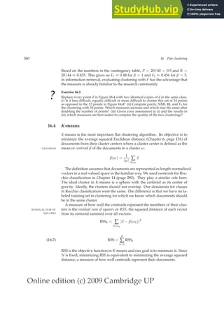
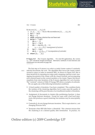
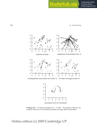
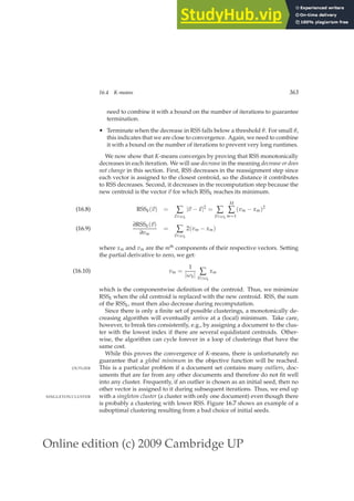
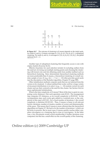

![Online edition (c) 2009 Cambridge UP
366 16 Flat clustering
2 4 6 8 10
1750
1800
1850
1900
1950
number of clusters
residual
sum
of
squares
◮ Figure 16.8 Estimated minimal residual sum of squares as a function of the num-
ber of clusters in K-means. In this clustering of 1203 Reuters-RCV1 documents, there
are two points where the d
RSSmin curve flattens: at 4 clusters and at 9 clusters. The
documents were selected from the categories China, Germany, Russia and Sports, so
the K = 4 clustering is closest to the Reuters classification.
A second type of criterion for cluster cardinality imposes a penalty for each
new cluster – where conceptually we start with a single cluster containing all
documents and then search for the optimal number of clusters K by succes-
sively incrementing K by one. To determine the cluster cardinality in this
way, we create a generalized objective function that combines two elements:
distortion, a measure of how much documents deviate from the prototype of
DISTORTION
their clusters (e.g., RSS for K-means); and a measure of model complexity. We
MODEL COMPLEXITY
interpret a clustering here as a model of the data. Model complexity in clus-
tering is usually the number of clusters or a function thereof. For K-means,
we then get this selection criterion for K:
K = arg min
K
[RSSmin(K) + λK]
(16.11)
where λ is a weighting factor. A large value of λ favors solutions with few
clusters. For λ = 0, there is no penalty for more clusters and K = N is the
best solution.](https://image.slidesharecdn.com/anintroductiontoinformationretrieval-230807170822-1d67eee0/85/An-Introduction-to-Information-Retrieval-pdf-391-320.jpg)
![Online edition (c) 2009 Cambridge UP
16.4 K-means 367
The obvious difficulty with Equation (16.11) is that we need to determine
λ. Unless this is easier than determining K directly, then we are back to
square one. In some cases, we can choose values of λ that have worked well
for similar data sets in the past. For example, if we periodically cluster news
stories from a newswire, there is likely to be a fixed value of λ that gives us
the right K in each successive clustering. In this application, we would not
be able to determine K based on past experience since K changes.
A theoretical justification for Equation (16.11) is the Akaike Information Cri-
AKAIKE INFORMATION
CRITERION terion or AIC, an information-theoretic measure that trades off distortion
against model complexity. The general form of AIC is:
AIC: K = arg min
K
[−2L(K) + 2q(K)]
(16.12)
where −L(K), the negative maximum log-likelihood of the data for K clus-
ters, is a measure of distortion and q(K), the number of parameters of a
model with K clusters, is a measure of model complexity. We will not at-
tempt to derive the AIC here, but it is easy to understand intuitively. The
first property of a good model of the data is that each data point is modeled
well by the model. This is the goal of low distortion. But models should
also be small (i.e., have low model complexity) since a model that merely
describes the data (and therefore has zero distortion) is worthless. AIC pro-
vides a theoretical justification for one particular way of weighting these two
factors, distortion and model complexity, when selecting a model.
For K-means, the AIC can be stated as follows:
AIC: K = arg min
K
[RSSmin(K) + 2MK]
(16.13)
Equation (16.13) is a special case of Equation (16.11) for λ = 2M.
To derive Equation (16.13) from Equation (16.12) observe that q(K) = KM
in K-means since each element of the K centroids is a parameter that can be
varied independently; and that L(K) = −(1/2)RSSmin(K) (modulo a con-
stant) if we view the model underlying K-means as a Gaussian mixture with
hard assignment, uniform cluster priors and identical spherical covariance
matrices (see Exercise 16.19).
The derivation of AIC is based on a number of assumptions, e.g., that the
data are independent and identically distributed. These assumptions are
only approximately true for data sets in information retrieval. As a conse-
quence, the AIC can rarely be applied without modification in text clustering.
In Figure 16.8, the dimensionality of the vector space is M ≈ 50,000. Thus,
2MK 50,000 dominates the smaller RSS-based term (d
RSSmin(1) 5000,
not shown in the figure) and the minimum of the expression is reached for
K = 1. But as we know, K = 4 (corresponding to the four classes China,](https://image.slidesharecdn.com/anintroductiontoinformationretrieval-230807170822-1d67eee0/85/An-Introduction-to-Information-Retrieval-pdf-392-320.jpg)


![Online edition (c) 2009 Cambridge UP
374 16 Flat clustering
ously with cluster assignment) is described by Cheeseman and Stutz (1996).
Two methods for determining cardinality without external criteria are pre-
sented by Tibshirani et al. (2001).
We only have space here for classical completely unsupervised clustering.
An important current topic of research is how to use prior knowledge to
guide clustering (e.g., Ji and Xu (2006)) and how to incorporate interactive
feedback during clustering (e.g., Huang and Mitchell (2006)). Fayyad et al.
(1998) propose an initialization for EM clustering. For algorithms that can
cluster very large data sets in one scan through the data see Bradley et al.
(1998).
The applications in Table 16.1 all cluster documents. Other information re-
trieval applications cluster words (e.g., Crouch 1988), contexts of words (e.g.,
Schütze and Pedersen 1995) or words and documents simultaneously (e.g.,
Tishby and Slonim 2000, Dhillon 2001, Zha et al. 2001). Simultaneous clus-
tering of words and documents is an example of co-clustering or biclustering.
CO-CLUSTERING
16.7 Exercises
? Exercise 16.7
Let Ω be a clustering that exactly reproduces a class structure C and Ω′ a clustering
that further subdivides some clusters in Ω. Show that I(Ω; C) = I(Ω′; C).
Exercise 16.8
Show that I(Ω; C) ≤ [H(Ω) + H(C)]/2.
Exercise 16.9
Mutual information is symmetric in the sense that its value does not change if the
roles of clusters and classes are switched: I(Ω; C) = I(C; Ω). Which of the other
three evaluation measures are symmetric in this sense?
Exercise 16.10
Compute RSS for the two clusterings in Figure 16.7.
Exercise 16.11
(i) Give an example of a set of points and three initial centroids (which need not be
members of the set of points) for which 3-means converges to a clustering with an
empty cluster. (ii) Can a clustering with an empty cluster be the global optimum with
respect to RSS?
Exercise 16.12
Download Reuters-21578. Discard documents that do not occur in one of the 10
classes acquisitions, corn, crude, earn, grain, interest, money-fx, ship, trade, and wheat.
Discard documents that occur in two of these 10 classes. (i) Compute a K-means clus-
tering of this subset into 10 clusters. There are a number of software packages that
implement K-means, such as WEKA (Witten and Frank 2005) and R (R Development
Core Team 2005). (ii) Compute purity, normalized mutual information, F1 and RI for](https://image.slidesharecdn.com/anintroductiontoinformationretrieval-230807170822-1d67eee0/85/An-Introduction-to-Information-Retrieval-pdf-399-320.jpg)
![Online edition (c) 2009 Cambridge UP
16.7 Exercises 375
the clustering with respect to the 10 classes. (iii) Compile a confusion matrix (Ta-
ble 14.5, page 308) for the 10 classes and 10 clusters. Identify classes that give rise to
false positives and false negatives.
Exercise 16.13
Prove that RSSmin(K) is monotonically decreasing in K.
Exercise 16.14
There is a soft version of K-means that computes the fractional membership of a doc-
ument in a cluster as a monotonically decreasing function of the distance ∆ from its
centroid, e.g., as e−∆. Modify reassignment and recomputation steps of hard K-means
for this soft version.
Exercise 16.15
In the last iteration in Table 16.3, document 6 is in cluster 2 even though it was the
initial seed for cluster 1. Why does the document change membership?
Exercise 16.16
The values of the parameters qmk in iteration 25 in Table 16.3 are rounded. What are
the exact values that EM will converge to?
Exercise 16.17
Perform a K-means clustering for the documents in Table 16.3. After how many
iterations does K-means converge? Compare the result with the EM clustering in
Table 16.3 and discuss the differences.
Exercise 16.18 [⋆ ⋆ ⋆]
Modify the expectation and maximization steps of EM for a Gaussian mixture. The
maximization step computes the maximum likelihood parameter estimates αk, ~
µk,
and Σk for each of the clusters. The expectation step computes for each vector a soft
assignment to clusters (Gaussians) based on their current parameters. Write down
the equations for Gaussian mixtures corresponding to Equations (16.16) and (16.17).
Exercise 16.19 [⋆ ⋆ ⋆]
Show that K-means can be viewed as the limiting case of EM for Gaussian mixtures
if variance is very small and all covariances are 0.
Exercise 16.20 [⋆ ⋆ ⋆]
The within-point scatter of a clustering is defined as ∑k
1
2 ∑~
xi∈ωk
∑~
xj∈ωk
|~
xi −~
xj|2. Show
WITHIN-POINT
SCATTER that minimizing RSS and minimizing within-point scatter are equivalent.
Exercise 16.21 [⋆ ⋆ ⋆]
Derive an AIC criterion for the multivariate Bernoulli mixture model from Equa-
tion (16.12).](https://image.slidesharecdn.com/anintroductiontoinformationretrieval-230807170822-1d67eee0/85/An-Introduction-to-Information-Retrieval-pdf-400-320.jpg)


![Online edition (c) 2009 Cambridge UP
380 17 Hierarchical clustering
in flat clustering. In those cases, the hierarchy needs to be cut at some point.
A number of criteria can be used to determine the cutting point:
• Cut at a prespecified level of similarity. For example, we cut the dendro-
gram at 0.4 if we want clusters with a minimum combination similarity
of 0.4. In Figure 17.1, cutting the diagram at y = 0.4 yields 24 clusters
(grouping only documents with high similarity together) and cutting it at
y = 0.1 yields 12 clusters (one large financial news cluster and 11 smaller
clusters).
• Cut the dendrogram where the gap between two successive combination
similarities is largest. Such large gaps arguably indicate “natural” clus-
terings. Adding one more cluster decreases the quality of the clustering
significantly, so cutting before this steep decrease occurs is desirable. This
strategy is analogous to looking for the knee in the K-means graph in Fig-
ure 16.8 (page 366).
• Apply Equation (16.11) (page 366):
K = arg min
K′
[RSS(K′
) + λK′
]
where K′ refers to the cut of the hierarchy that results in K′ clusters, RSS is
the residual sum of squares and λ is a penalty for each additional cluster.
Instead of RSS, another measure of distortion can be used.
• As in flat clustering, we can also prespecify the number of clusters K and
select the cutting point that produces K clusters.
A simple, naive HAC algorithm is shown in Figure 17.2. We first compute
the N × N similarity matrix C. The algorithm then executes N − 1 steps
of merging the currently most similar clusters. In each iteration, the two
most similar clusters are merged and the rows and columns of the merged
cluster i in C are updated.2 The clustering is stored as a list of merges in
A. I indicates which clusters are still available to be merged. The function
SIM(i, m, j) computes the similarity of cluster j with the merge of clusters i
and m. For some HAC algorithms, SIM(i, m, j) is simply a function of C[j][i]
and C[j][m], for example, the maximum of these two values for single-link.
We will now refine this algorithm for the different similarity measures
of single-link and complete-link clustering (Section 17.2) and group-average
and centroid clustering (Sections 17.3 and 17.4). The merge criteria of these
four variants of HAC are shown in Figure 17.3.
2. We assume that we use a deterministic method for breaking ties, such as always choose the
merge that is the first cluster with respect to a total ordering of the subsets of the document set
D.](https://image.slidesharecdn.com/anintroductiontoinformationretrieval-230807170822-1d67eee0/85/An-Introduction-to-Information-Retrieval-pdf-405-320.jpg)
![Online edition (c) 2009 Cambridge UP
17.1 Hierarchical agglomerative clustering 381
SIMPLEHAC(d1, . . . , dN)
1 for n ← 1 to N
2 do for i ← 1 to N
3 do C[n][i] ← SIM(dn, di)
4 I[n] ← 1 (keeps track of active clusters)
5 A ← [] (assembles clustering as a sequence of merges)
6 for k ← 1 to N − 1
7 do hi, mi ← arg max{hi,mi:i6=m∧I[i]=1∧I[m]=1} C[i][m]
8 A.APPEND(hi, mi) (store merge)
9 for j ← 1 to N
10 do C[i][j] ← SIM(i, m, j)
11 C[j][i] ← SIM(i, m, j)
12 I[m] ← 0 (deactivate cluster)
13 return A
◮ Figure 17.2 A simple, but inefficient HAC algorithm.
b
b
b
b
(a) single-link: maximum similarity
b
b
b
b
(b) complete-link: minimum similarity
b
b
b
b
(c) centroid: average inter-similarity
b
b
b
b
(d) group-average: average of all similarities
◮ Figure 17.3 The different notions of cluster similarity used by the four HAC al-
gorithms. An inter-similarity is a similarity between two documents from different
clusters.](https://image.slidesharecdn.com/anintroductiontoinformationretrieval-230807170822-1d67eee0/85/An-Introduction-to-Information-Retrieval-pdf-406-320.jpg)
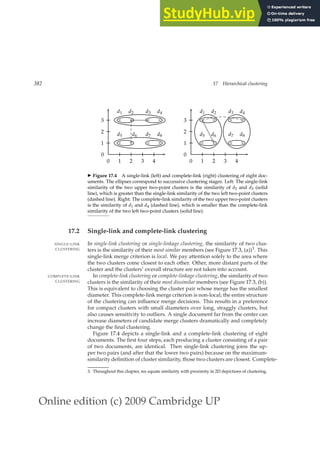

![Online edition (c) 2009 Cambridge UP
17.2 Single-link and complete-link clustering 385
0 1 2 3 4 5 6 7
0
1 ×
d1
×
d2
×
d3
×
d4
×
d5
◮ Figure 17.7 Outliers in complete-link clustering. The five documents have
the x-coordinates 1 + 2ǫ, 4, 5 + 2ǫ, 6 and 7 − ǫ. Complete-link clustering cre-
ates the two clusters shown as ellipses. The most intuitive two-cluster cluster-
ing is {{d1}, {d2, d3, d4, d5}}, but in complete-link clustering, the outlier d1 splits
{d2, d3, d4, d5} as shown.
distances without regard to the overall shape of the emerging cluster. This
effect is called chaining.
CHAINING
The chaining effect is also apparent in Figure 17.1. The last eleven merges
of the single-link clustering (those above the 0.1 line) add on single docu-
ments or pairs of documents, corresponding to a chain. The complete-link
clustering in Figure 17.5 avoids this problem. Documents are split into two
groups of roughly equal size when we cut the dendrogram at the last merge.
In general, this is a more useful organization of the data than a clustering
with chains.
However, complete-link clustering suffers from a different problem. It
pays too much attention to outliers, points that do not fit well into the global
structure of the cluster. In the example in Figure 17.7 the four documents
d2, d3, d4, d5 are split because of the outlier d1 at the left edge (Exercise 17.1).
Complete-link clustering does not find the most intuitive cluster structure in
this example.
17.2.1 Time complexity of HAC
The complexity of the naive HAC algorithm in Figure 17.2 is Θ(N3) because
we exhaustively scan the N × N matrix C for the largest similarity in each of
N − 1 iterations.
For the four HAC methods discussed in this chapter a more efficient algo-
rithm is the priority-queue algorithm shown in Figure 17.8. Its time complex-
ity is Θ(N2 log N). The rows C[k] of the N × N similarity matrix C are sorted
in decreasing order of similarity in the priority queues P. P[k].MAX() then
returns the cluster in P[k] that currently has the highest similarity with ωk,
where we use ωk to denote the kth
cluster as in Chapter 16. After creating the
merged cluster of ωk1
and ωk2
, ωk1
is used as its representative. The function
SIM computes the similarity function for potential merge pairs: largest simi-
larity for single-link, smallest similarity for complete-link, average similarity
for GAAC (Section 17.3), and centroid similarity for centroid clustering (Sec-](https://image.slidesharecdn.com/anintroductiontoinformationretrieval-230807170822-1d67eee0/85/An-Introduction-to-Information-Retrieval-pdf-410-320.jpg)
![Online edition (c) 2009 Cambridge UP
386 17 Hierarchical clustering
EFFICIENTHAC(~
d1, . . . , ~
dN)
1 for n ← 1 to N
2 do for i ← 1 to N
3 do C[n][i].sim ← ~
dn · ~
di
4 C[n][i].index ← i
5 I[n] ← 1
6 P[n] ← priority queue for C[n] sorted on sim
7 P[n].DELETE(C[n][n]) (don’t want self-similarities)
8 A ← []
9 for k ← 1 to N − 1
10 do k1 ← arg max{k:I[k]=1} P[k].MAX().sim
11 k2 ← P[k1].MAX().index
12 A.APPEND(hk1, k2i)
13 I[k2] ← 0
14 P[k1] ← []
15 for each i with I[i] = 1 ∧ i 6= k1
16 do P[i].DELETE(C[i][k1])
17 P[i].DELETE(C[i][k2])
18 C[i][k1].sim ← SIM(i, k1, k2)
19 P[i].INSERT(C[i][k1])
20 C[k1][i].sim ← SIM(i, k1, k2)
21 P[k1].INSERT(C[k1][i])
22 return A
clustering algorithm SIM(i, k1, k2)
single-link max(SIM(i, k1), SIM(i, k2))
complete-link min(SIM(i, k1), SIM(i, k2))
centroid ( 1
Nm
~
vm) · ( 1
Ni
~
vi)
group-average 1
(Nm+Ni)(Nm+Ni−1)
[(~
vm +~
vi)2 − (Nm + Ni)]
compute C[5]
1 2 3 4 5
0.2 0.8 0.6 0.4 1.0
create P[5] (by sorting)
2 3 4 1
0.8 0.6 0.4 0.2
merge 2 and 3, update
similarity of 2, delete 3
2 4 1
0.3 0.4 0.2
delete and reinsert 2
4 2 1
0.4 0.3 0.2
◮ Figure 17.8 The priority-queue algorithm for HAC. Top: The algorithm. Center:
Four different similarity measures. Bottom: An example for processing steps 6 and
16–19. This is a made up example showing P[5] for a 5 × 5 matrix C.](https://image.slidesharecdn.com/anintroductiontoinformationretrieval-230807170822-1d67eee0/85/An-Introduction-to-Information-Retrieval-pdf-411-320.jpg)
![Online edition (c) 2009 Cambridge UP
17.2 Single-link and complete-link clustering 387
SINGLELINKCLUSTERING(d1, . . . , dN)
1 for n ← 1 to N
2 do for i ← 1 to N
3 do C[n][i].sim ← SIM(dn, di)
4 C[n][i].index ← i
5 I[n] ← n
6 NBM[n] ← arg maxX∈{C[n][i]:n6=i} X.sim
7 A ← []
8 for n ← 1 to N − 1
9 do i1 ← arg max{i:I[i]=i} NBM[i].sim
10 i2 ← I[NBM[i1].index]
11 A.APPEND(hi1, i2i)
12 for i ← 1 to N
13 do if I[i] = i ∧ i 6= i1 ∧ i 6= i2
14 then C[i1][i].sim ← C[i][i1].sim ← max(C[i1][i].sim, C[i2][i].sim)
15 if I[i] = i2
16 then I[i] ← i1
17 NBM[i1] ← arg maxX∈{C[i1][i]:I[i]=i∧i6=i1} X.sim
18 return A
◮ Figure 17.9 Single-link clustering algorithm using an NBM array. After merging
two clusters i1 and i2, the first one (i1) represents the merged cluster. If I[i] = i, then i
is the representative of its current cluster. If I[i] 6= i, then i has been merged into the
cluster represented by I[i] and will therefore be ignored when updating NBM[i1].
tion 17.4). We give an example of how a row of C is processed (Figure 17.8,
bottom panel). The loop in lines 1–7 is Θ(N2) and the loop in lines 9–21 is
Θ(N2 log N) for an implementation of priority queues that supports deletion
and insertion in Θ(log N). The overall complexity of the algorithm is there-
fore Θ(N2 log N). In the definition of the function SIM, ~
vm and ~
vi are the
vector sums of ωk1
∪ ωk2
and ωi, respectively, and Nm and Ni are the number
of documents in ωk1
∪ ωk2
and ωi, respectively.
The argument of EFFICIENTHAC in Figure 17.8 is a set of vectors (as op-
posed to a set of generic documents) because GAAC and centroid clustering
(Sections 17.3 and 17.4) require vectors as input. The complete-link version
of EFFICIENTHAC can also be applied to documents that are not represented
as vectors.
For single-link, we can introduce a next-best-merge array (NBM) as a fur-
ther optimization as shown in Figure 17.9. NBM keeps track of what the best
merge is for each cluster. Each of the two top level for-loops in Figure 17.9
are Θ(N2), thus the overall complexity of single-link clustering is Θ(N2).](https://image.slidesharecdn.com/anintroductiontoinformationretrieval-230807170822-1d67eee0/85/An-Introduction-to-Information-Retrieval-pdf-412-320.jpg)
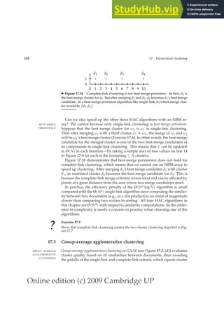
![Online edition (c) 2009 Cambridge UP
17.3 Group-average agglomerative clustering 389
similarity with the similarity of a single pair of documents. GAAC is also
called group-average clustering and average-link clustering. GAAC computes
the average similarity SIM-GA of all pairs of documents, including pairs from
the same cluster. But self-similarities are not included in the average:
SIM-GA(ωi, ωj) =
1
(Ni + Nj)(Ni + Nj − 1) ∑
dm∈ωi∪ωj
∑
dn∈ωi∪ωj,dn6=dm
~
dm · ~
dn
(17.1)
where ~
d is the length-normalized vector of document d, · denotes the dot
product, and Ni and Nj are the number of documents in ωi and ωj, respec-
tively.
The motivation for GAAC is that our goal in selecting two clusters ωi
and ωj as the next merge in HAC is that the resulting merge cluster ωk =
ωi ∪ ωj should be coherent. To judge the coherence of ωk, we need to look
at all document-document similarities within ωk, including those that occur
within ωi and those that occur within ωj.
We can compute the measure SIM-GA efficiently because the sum of indi-
vidual vector similarities is equal to the similarities of their sums:
∑
dm∈ωi
∑
dn∈ωj
(~
dm · ~
dn) = ( ∑
dm∈ωi
~
dm) · ( ∑
dn∈ωj
~
dn)
(17.2)
With (17.2), we have:
SIM-GA(ωi, ωj) =
1
(Ni + Nj)(Ni + Nj − 1)
[( ∑
dm∈ωi∪ωj
~
dm)2
− (Ni + Nj)]
(17.3)
The term (Ni + Nj) on the right is the sum of Ni + Nj self-similarities of value
1.0. With this trick we can compute cluster similarity in constant time (as-
suming we have available the two vector sums ∑dm∈ωi
~
dm and ∑dm∈ωj
~
dm)
instead of in Θ(NiNj). This is important because we need to be able to com-
pute the function SIM on lines 18 and 20 in EFFICIENTHAC (Figure 17.8)
in constant time for efficient implementations of GAAC. Note that for two
singleton clusters, Equation (17.3) is equivalent to the dot product.
Equation (17.2) relies on the distributivity of the dot product with respect
to vector addition. Since this is crucial for the efficient computation of a
GAAC clustering, the method cannot be easily applied to representations of
documents that are not real-valued vectors. Also, Equation (17.2) only holds
for the dot product. While many algorithms introduced in this book have
near-equivalent descriptions in terms of dot product, cosine similarity and
Euclidean distance (cf. Section 14.1, page 291), Equation (17.2) can only be
expressed using the dot product. This is a fundamental difference between
single-link/complete-link clustering and GAAC. The first two only require a](https://image.slidesharecdn.com/anintroductiontoinformationretrieval-230807170822-1d67eee0/85/An-Introduction-to-Information-Retrieval-pdf-414-320.jpg)
![Online edition (c) 2009 Cambridge UP
390 17 Hierarchical clustering
square matrix of similarities as input and do not care how these similarities
were computed.
To summarize, GAAC requires (i) documents represented as vectors, (ii)
length normalization of vectors, so that self-similarities are 1.0, and (iii) the
dot product as the measure of similarity between vectors and sums of vec-
tors.
The merge algorithms for GAAC and complete-link clustering are the same
except that we use Equation (17.3) as similarity function in Figure 17.8. There-
fore, the overall time complexity of GAAC is the same as for complete-link
clustering: Θ(N2 log N). Like complete-link clustering, GAAC is not best-
merge persistent (Exercise 17.6). This means that there is no Θ(N2) algorithm
for GAAC that would be analogous to the Θ(N2) algorithm for single-link in
Figure 17.9.
We can also define group-average similarity as including self-similarities:
SIM-GA
′
(ωi, ωj) =
1
(Ni+Nj)2
( ∑
dm∈ωi∪ωj
~
dm)2
=
1
Ni+Nj
∑
dm∈ωi∪ωj
[~
dm ·~
µ(ωi∪ωj)]
(17.4)
where the centroid ~
µ(ω) is defined as in Equation (14.1) (page 292). This
definition is equivalent to the intuitive definition of cluster quality as average
similarity of documents ~
dm to the cluster’s centroid ~
µ.
Self-similarities are always equal to 1.0, the maximum possible value for
length-normalized vectors. The proportion of self-similarities in Equation (17.4)
is i/i2 = 1/i for a cluster of size i. This gives an unfair advantage to small
clusters since they will have proportionally more self-similarities. For two
documents d1, d2 with a similarity s, we have SIM-GA′(d1, d2) = (1 + s)/2.
In contrast, SIM-GA(d1, d2) = s ≤ (1 + s)/2. This similarity SIM-GA(d1, d2)
of two documents is the same as in single-link, complete-link and centroid
clustering. We prefer the definition in Equation (17.3), which excludes self-
similarities from the average, because we do not want to penalize large clus-
ters for their smaller proportion of self-similarities and because we want a
consistent similarity value s for document pairs in all four HAC algorithms.
?
Exercise 17.2
Apply group-average clustering to the points in Figures 17.6 and 17.7. Map them onto
the surface of the unit sphere in a three-dimensional space to get length-normalized
vectors. Is the group-average clustering different from the single-link and complete-
link clusterings?](https://image.slidesharecdn.com/anintroductiontoinformationretrieval-230807170822-1d67eee0/85/An-Introduction-to-Information-Retrieval-pdf-415-320.jpg)
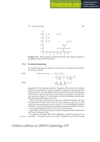
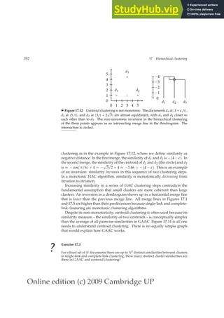
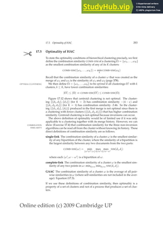
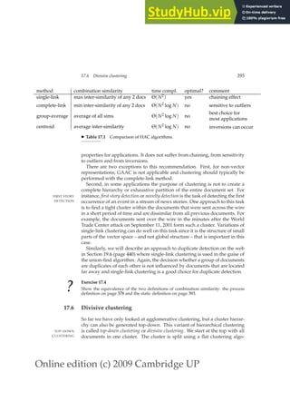
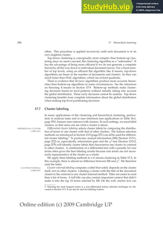
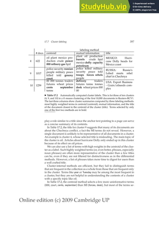
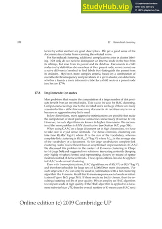


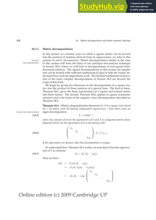


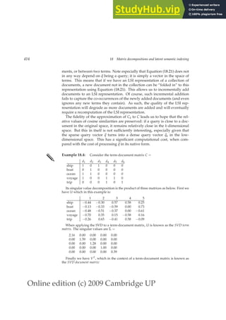


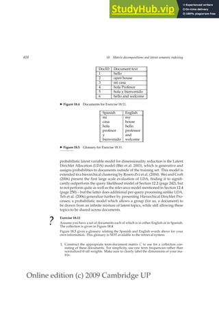


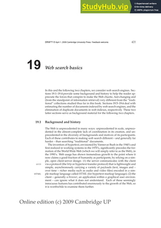


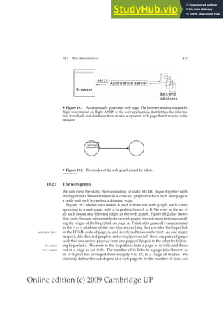
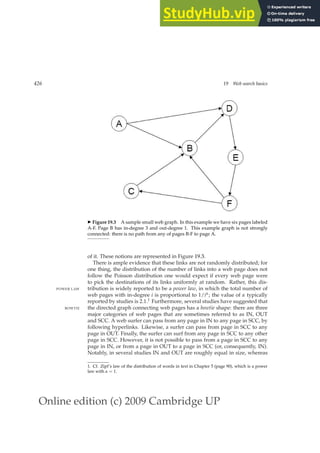
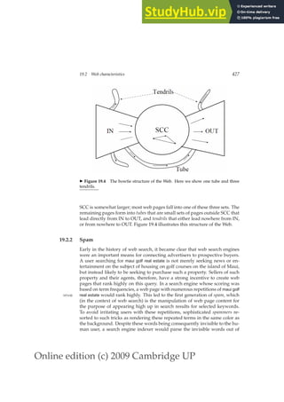
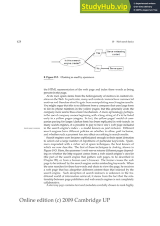
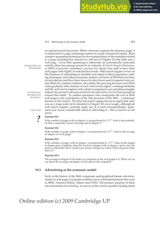

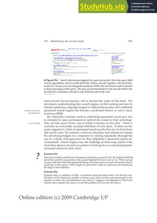

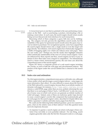
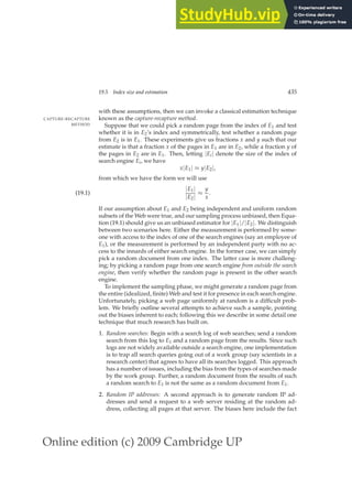

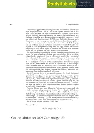


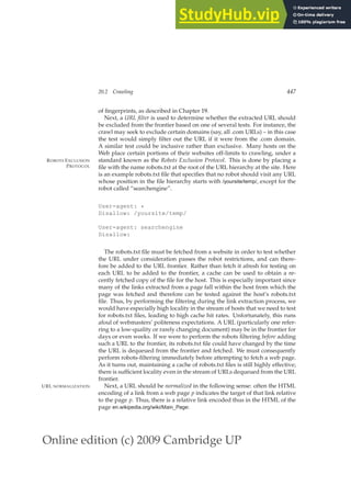
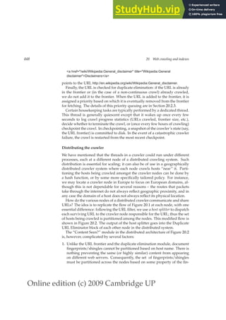
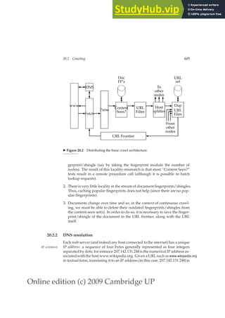


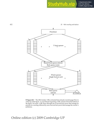
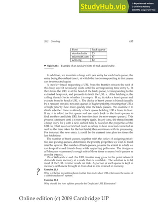

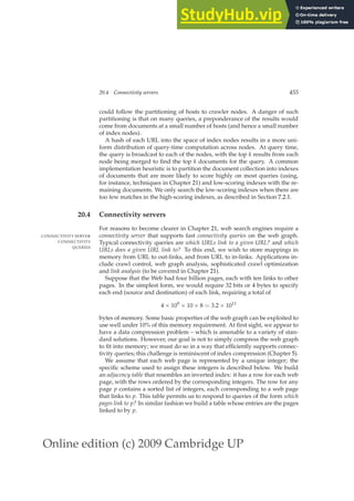
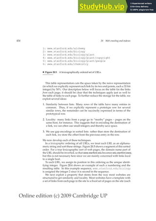


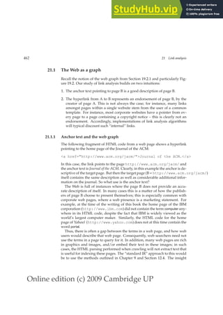


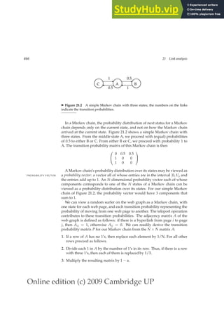


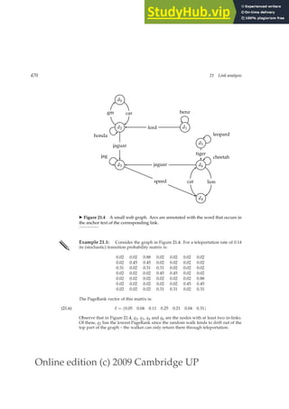
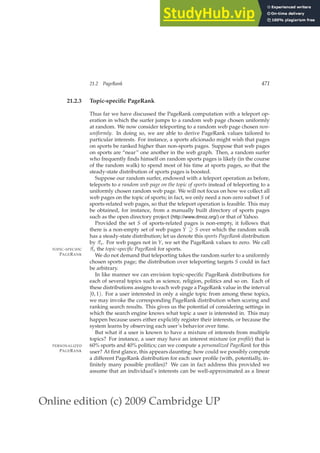
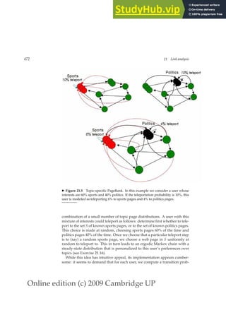

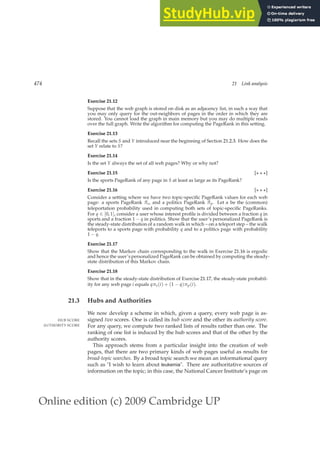
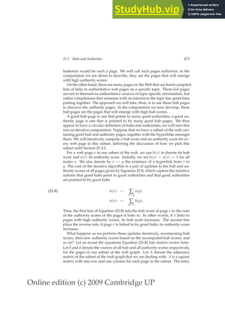


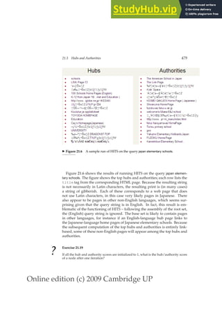


This document provides a draft table of contents for the book "An Introduction to Information Retrieval" by Christopher Manning, Prabhakar Raghavan, and Hinrich Schütze. The book covers topics such as Boolean retrieval models, term vocabularies, index construction, scoring and weighting models, evaluation, query expansion, XML retrieval, probabilistic models, language models, text classification, clustering, and web search. The draft table of contents lists 18 chapters and their brief contents.