Downloaded 75 times
![Graph Indexing Techniques
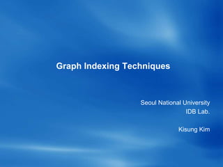
Target Database Query Type
GraphGrep
[Shasha et al., PODS’02]
Collection DB Exact Feature(Path) based index
gIndex
[Yan et al., SIGMOD’04]
Collection DB Exact Feature(Graph) based index
Grafil
[Yan et al., SIGMOD’05]
Collection DB Exact & Similarity Feature based similarity search
C-tree
[He and Singh, ICDE’06]
Collection DB Exact & Similarity Closure based index
QuickSI
[Shang et al., VLDB’08]
Collection DB Exact Verification algorithm
Tale
[Tian and Patel, ICDE’08]
Collection DB Exact & Similarity Similarity search using node index
GraphQL
[He and Singh, SIGMOD’08]
Large graphs Exact Node indexing
Spath
[Zhao and Han, VLDB’10]
Large graphs Exact
Node indexing using
neighborhood information
7/50](https://image.slidesharecdn.com/surveygraphindexing-170305222417/85/Survey-of-Graph-Indexing-7-320.jpg)
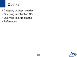
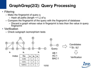
![GraphGrep(1/2) [Shasha et al. PODS’02]
• First work adopts the filtering-and-verification framework
• Path-based index
– Fingerprint of database
– Enumerate the set of all paths(length <= L) of all graphs in DB
– For each path, the number of occurrences in each graphs are stored in
hash table
B
A
C
B
B
A
C
B
D
E
C
A B
B
C
Key g1 g2 g3
h(CA) 1 0 1
…
h(ABCB) 2 2 0
g1 g2 g3 Index
9/50](https://image.slidesharecdn.com/surveygraphindexing-170305222417/85/Survey-of-Graph-Indexing-9-320.jpg)
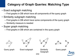
![gIndex(1/6) [Yan et al., SIGMOD’04]
• Path-based approach has week points
– Path is too simple: structural information is lost
– There are too many paths: the set of paths in a graph database usually
is huge
• Solution
– Use graph structure instead of path as the basic index feature
c c c c
c c
c c
c c
c c
c c
c c
c c
c c
Sample Database
c
c c
c
c
c
Query
c c c
c c c
Paths in Query Graph
Cannot Filter Any
Graphs
In Database
11/50](https://image.slidesharecdn.com/surveygraphindexing-170305222417/85/Survey-of-Graph-Indexing-11-320.jpg)
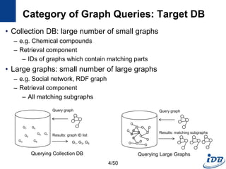
![a
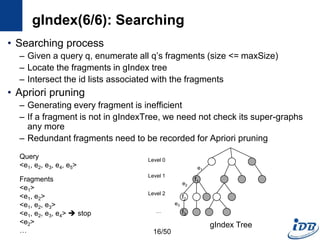
gIndex(5/6): gIndex Tree
• Use graph serialization method
– For fast graph isomorphism checking during index search
– DFS coding [Yan et al. ICDM’02]
– Translate a graph into a unique edge sequence
• gIndex Tree
– Prefix tree which consists of the edge sequences of discriminative fragments
– Record all size-n discriminative fragments in level n
– Black nodes discriminative fragments
– Have ID lists: the ids of graphs containing fi
– White nodes redundant fragments; for Apriori pruning
X
X
Z Y
b
a
ba
X
X
Z Y
b
ba
v0
v1
v2 v3
DFS Coding
<(v0,v1),(v1,v2),(v2,v0),(v1,v3)>
f1
f2
f3
e1
e2
e3
Level 0
Level 1
Level 2
…
gIndex Tree
15/50](https://image.slidesharecdn.com/surveygraphindexing-170305222417/85/Survey-of-Graph-Indexing-15-320.jpg)
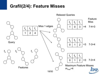
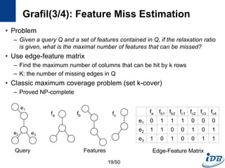
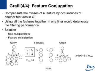
![Grafil(1/4) [Yan et al., SIGMOD’05]
• Subgraph similarity search
• Feature-based approach
• Similarity search using relaxed queries
– Relax a query by deletion of k edges
– Missed edges incur missed features
• Main question
– What is the maximum missed features(𝑚 𝑚𝑎𝑥) when relaxing a query
with k missed edges?
Feature Vector
G1 {u1, u2, …, un}
G2
…
Gn
Subgraph exact search
Subgraph similarity search
𝑓𝑜𝑟 1 ≤ 𝑖 ≤ 𝑛, 𝑢𝑖 ≥ 𝑣𝑖
{v1, v2, …, vn}
𝑟 𝑢𝑖, 𝑣𝑖 =
0, 𝑖𝑓𝑢𝑖 ≥ 𝑣𝑖
𝑢𝑖 − 𝑣𝑖, 𝑜𝑡ℎ𝑒𝑟𝑤𝑖𝑠𝑒
𝑖=1
𝑛
𝑟 𝑢𝑖, 𝑣𝑖 ≤ 𝑚 𝑚𝑎𝑥
Query
17/50](https://image.slidesharecdn.com/surveygraphindexing-170305222417/85/Survey-of-Graph-Indexing-17-320.jpg)
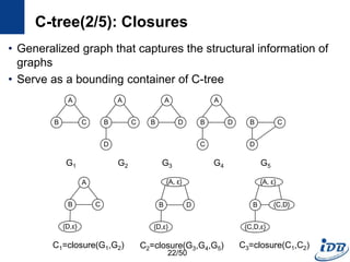
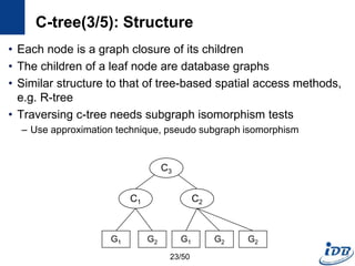
![C-tree(1/5) [He and Singh, ICDE’06]
• Closure-tree
– Tree-based index
– Each node has graph closure of its descendants
– Support subgraph queries and similarity queries
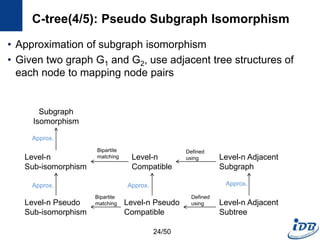
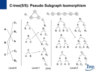
• Pseudo subgraph isomorphism
– Perform pairwise graph comparisons using heuristic techniques
– Produce candidate answers within a polynomial time
C-tree
Query
Graph
Candidate
Graphs
21/50](https://image.slidesharecdn.com/surveygraphindexing-170305222417/85/Survey-of-Graph-Indexing-21-320.jpg)
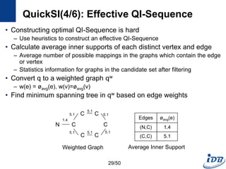
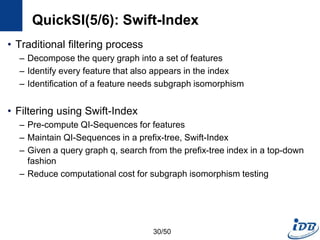
![QuickSI(1/6) [Shang et al., VLDB’08]
• Main paradigm for processing graph containment queries
– Filtering-and-verification framework
• Verification techniques
– Subgraph isomorphism testing
– Existing techniques are not efficient especially when the query graph
size becomes large
• Develop efficient verification techniques
26/50](https://image.slidesharecdn.com/surveygraphindexing-170305222417/85/Survey-of-Graph-Indexing-26-320.jpg)
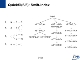
![QuickSI(2/6): QI-Sequence
• A Sequence that represents a rooted spanning tree for a query q
– Encode a graph for efficient subgraph isomorphism testing
– Encode search order and topological information
– Have spanning entries and extra entries
• Spanning entry, Ti
– Keep basic information of the spanning tree
– Ti.v: record a vertex vk in a query graph q
– [Ti.p, Ti.l] : parent vertex and label of Ti.v
• Extra entry, Rij
– Extra topology information
– Degree constraint [deg : d] : the degree of Ti.v
– Extra edge [edge : j] : edge that doesn’t appear in the spanning tree
27/50](https://image.slidesharecdn.com/surveygraphindexing-170305222417/85/Survey-of-Graph-Indexing-27-320.jpg)
![QuickSI(3/6): QI-Sequence
• Several QI-Sequences of one query graph, q
– Different search spaces when processing subgraph isomorphism testing
N C
C C
C
C C
Type [Ti.p, Ti.l] Ti.v
T1 [0, N] v1
T2 [1, C] v2
R21 [deg : 3]
T3 [2, C] v3
T4 [3, C] v4
T5 [4, C] v5
T6 [5, C] v6
T7 [6, C] v7
R71 [edge : 2]
Type [Ti.p, Ti.l] Ti.v
T1 [0, C] v4
T2 [1, C] v5
R61 [edge : 3]
T3 [2, C] v3
T4 [3, C] v6
T5 [4, C] v7
T6 [5, C] v2
T7 [6, C] v1
R61 [deg : 3]
Query
QI-Sequence, SEQq QI-Sequence, SEQq’
28/50](https://image.slidesharecdn.com/surveygraphindexing-170305222417/85/Survey-of-Graph-Indexing-28-320.jpg)
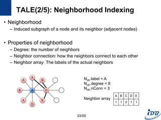
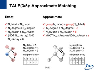
![TALE(1/5) [Tian and Patel, ICDE’08]
• Motivation
– Need approximate graph matching
– Supporting large queries is more and more desired
• TALE (A Tool for Approximate Large Graph Matching)
– A Novel Disk-based Indexing Method
– High pruning power
– Linear index size with the database size
– Index-based matching algorithm
– Significantly outperforms existing methods
– Gracefully handles large queries and databases
32/50](https://image.slidesharecdn.com/surveygraphindexing-170305222417/85/Survey-of-Graph-Indexing-32-320.jpg)
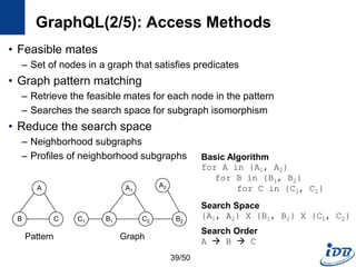
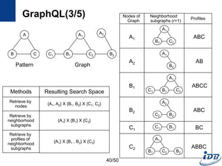
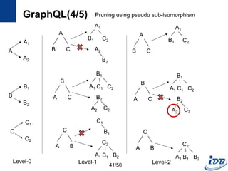
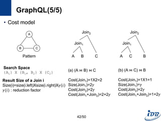
![GraphQL(1/5) [He and Singh, SIGMOD’08]
• Motivation
– Need a language to query and manipulate graphs with arbitrary attributes
and structures
– Native access methods that exploit graph structural information
• Formal language for graphs
– Notion for manipulating graph structures
– Basis of graph query language
– Concatenation, disjunction, repetition
• Graph query language
– Subgraph isomorphism + predicate evaluation
graph G1 {
node v1, v2, v3;
edge e1 (v1, v2);
edge e2 (v2, v3);
edge e3 (v3, v1);
}
v1
v2 v3
e1 e3
e2
graph P {
node v1, v2;
edge e1 (v1, v2);
} where v1.name = “A”
and v2.year > 2000;
Graph motif Graph pattern
38/50](https://image.slidesharecdn.com/surveygraphindexing-170305222417/85/Survey-of-Graph-Indexing-38-320.jpg)
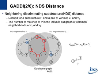
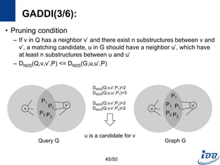
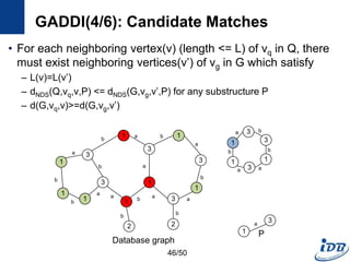
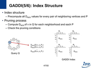
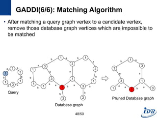
![GADDI(1/6) [Zhang et al., EDBT’09]
• Employ novel indexing method, NDS distance
– Capture the local graph structure between each pair of vertices
– More pruning power than indexes which are based on information of one
vertex
• Matching algorithm based on two-way pruning
– Candidate matching using NDS distance
– Remove impossible vertices after some vertices are matched
43/50](https://image.slidesharecdn.com/surveygraphindexing-170305222417/85/Survey-of-Graph-Indexing-43-320.jpg)
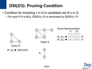
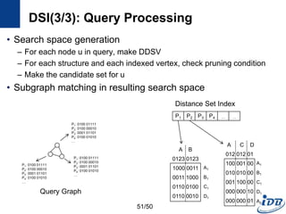
![DSI(1/3) [Kou et al., WAIM’10]
• Discriminative structure
• Distance set
– Distinct distances of all the path between a vertex, v and substructures
in k-N(v)
– The path must not contain an edge in P
49/50
A1
B1
D1
C1
A2
A
B
Graph G
P1
A1
B1
Distance (k=3)
P1.A A1 : 0
P1.B A1 : 2, 3
P1.A A2 : 2, 3
P1.B A2 : 3, (4)
Vector Representation
A B
0123 0123
(P1,A1) 1000 0011
(P1,A2) 0011 0001](https://image.slidesharecdn.com/surveygraphindexing-170305222417/85/Survey-of-Graph-Indexing-49-320.jpg)
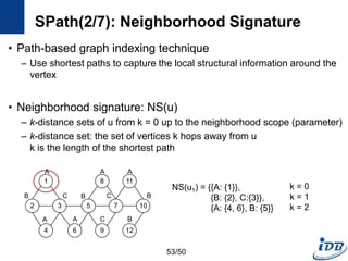
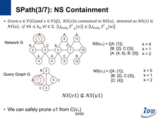
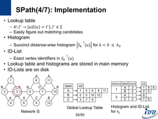
![SPath(1/7) [Zhao and Han, VLDB’10]
• Problems of previous graph matching methods
– Designed on special graphs
– Limited guarantee on query performance and scalability support
– Lack of scalable graph indexing mechanisms and cost-effective graph
query optimizer
• SPath
– Compact indexing structure using local structural information of vertices:
neighborhood signatures
– Query processing: vertex-at-a-time to path-at-a-time
• Target graph
– Connected, undirected simple graphs with no edge weights
– Labeled vertices
52/50](https://image.slidesharecdn.com/surveygraphindexing-170305222417/85/Survey-of-Graph-Indexing-52-320.jpg)
![References
• [Shasha et al., PODS’02] Dennis Shasha, Jaso T. L. Wang, Rosalba Giugno,
Algorithmics and Applications of Tree and Graph Searching. PODS, 2002.
• [Yan et al., SIGMOD’04] Xifeng Yan, Philip S. Yu, Jiawei Han, Graph Indexing:
A Frequent Structure-based Approach. SIGMOD, 2004.
• [Yan et al., SIGMOD’05] Xifeng Yan, Philip S. Yu, Jiawei Han, Substructure
Similarity Search in Graph Databases. SIGMOD, 2005.
• [Tian and Patel, ICDE’08] Yuanyuan Tian , Jignesh M. Patel. TALE: A Tool for
Approximate Large Graph Matching. ICDE, 2008.
• [He and Singh, SIGMOD’08] Huahai He, Ambuj K. Singh. Graphs-at-a-time:
query language and access methods for graph databases. SIGMOD, 2008.
• [Zhao and Han, VLDB’10] Peiziang Zhao, Jiawei Han. On Graph Query
Optimization in Large Networks. VLDB, 2010.
• [He and Singh, ICDE’06] Huahai He, Ambuj K. Singh, Closure-Tree: An Index
Structure for Graph Queries. ICDE, 2006
• [Shang et al., VLDB’08] Haichuan Shang, Ying Zhang, Xuemin Lin, Jeffrey Xu
Yu, Taming Verification Hardness: An Efficient Algorithm for Testing Subgraph
Isomorphism. VLDB, 2008
59/50](https://image.slidesharecdn.com/surveygraphindexing-170305222417/85/Survey-of-Graph-Indexing-59-320.jpg)
![References
• [Zhang et al., EDBT’09] Shijie Zhang, Shirong Li, Jiong Yang,
GADDI: Distance Index based Subgraph Matching in
Biological Networks. EDBT, 2009
• [Zhang et al., CIKM’10] Shijie Zhang, Shirong Li, Jiong Yang,
SUMMA: Subgraph Matching in Massive Graphs. CIKM, 2010
• [Kou et al., WAIM’10] Yubo Kou, Yukun Li, Xiaofeng Meng,
DSI: A Method for Indexing Large Graphs Using Distance Set.
WAIM, 2010
60/50](https://image.slidesharecdn.com/surveygraphindexing-170305222417/85/Survey-of-Graph-Indexing-60-320.jpg)

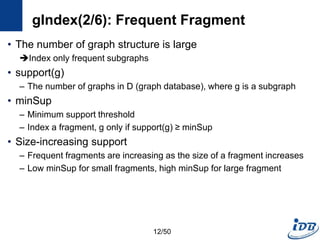
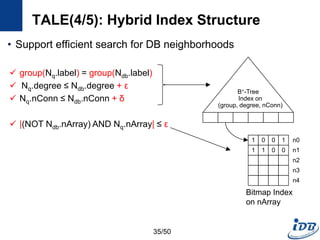
The document discusses techniques for indexing and querying graph data. It begins by categorizing graph queries as exact subgraph matching, similarity subgraph matching, or super graph matching. It then describes querying approaches for collection databases containing many small graphs versus large singular graphs. The document proceeds to summarize several graph indexing techniques including GraphGrep, gIndex, Grafil, C-tree, QuickSI, and others. It focuses on filtering techniques used to reduce the number of verification steps in subgraph matching queries over graph databases.


![[DSC Europe 25] Marcos Heidemann - Beyond the Hype: Making AI Coding Assistan...](https://cdn.slidesharecdn.com/ss_thumbnails/eexkhvldrjsopspdjbur-marcos-heidemann-beyond-the-hype-getting-real-value-out-of-ai-assisted-coding-260121115910-7e9d41ec-thumbnail.jpg?width=640&height=640&fit=bounds)


![[DSC Europe 25] Bojan Djuricic - Predictive Design Process.pdf](https://cdn.slidesharecdn.com/ss_thumbnails/5awdrbedqdek3gqu2ezy-4-the-predictive-design-bojan-djuricic-260120105856-6c399e9b-thumbnail.jpg?width=640&height=640&fit=bounds)
![[DSC Europe 25] Borko Kozomora - Optimizing business workflows with advances ...](https://cdn.slidesharecdn.com/ss_thumbnails/hbgekyb0txw0xpo4yfml-borko-kozomora-leading-ai-transformation-260122103838-cc29ee38-thumbnail.jpg?width=640&height=640&fit=bounds)