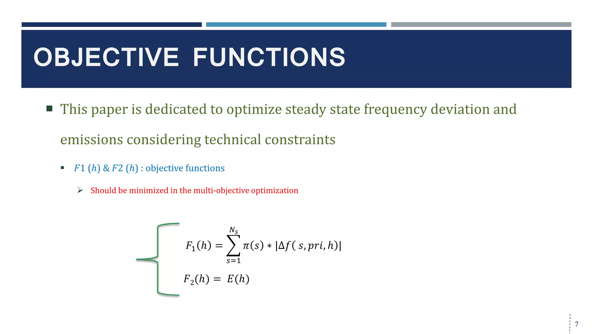
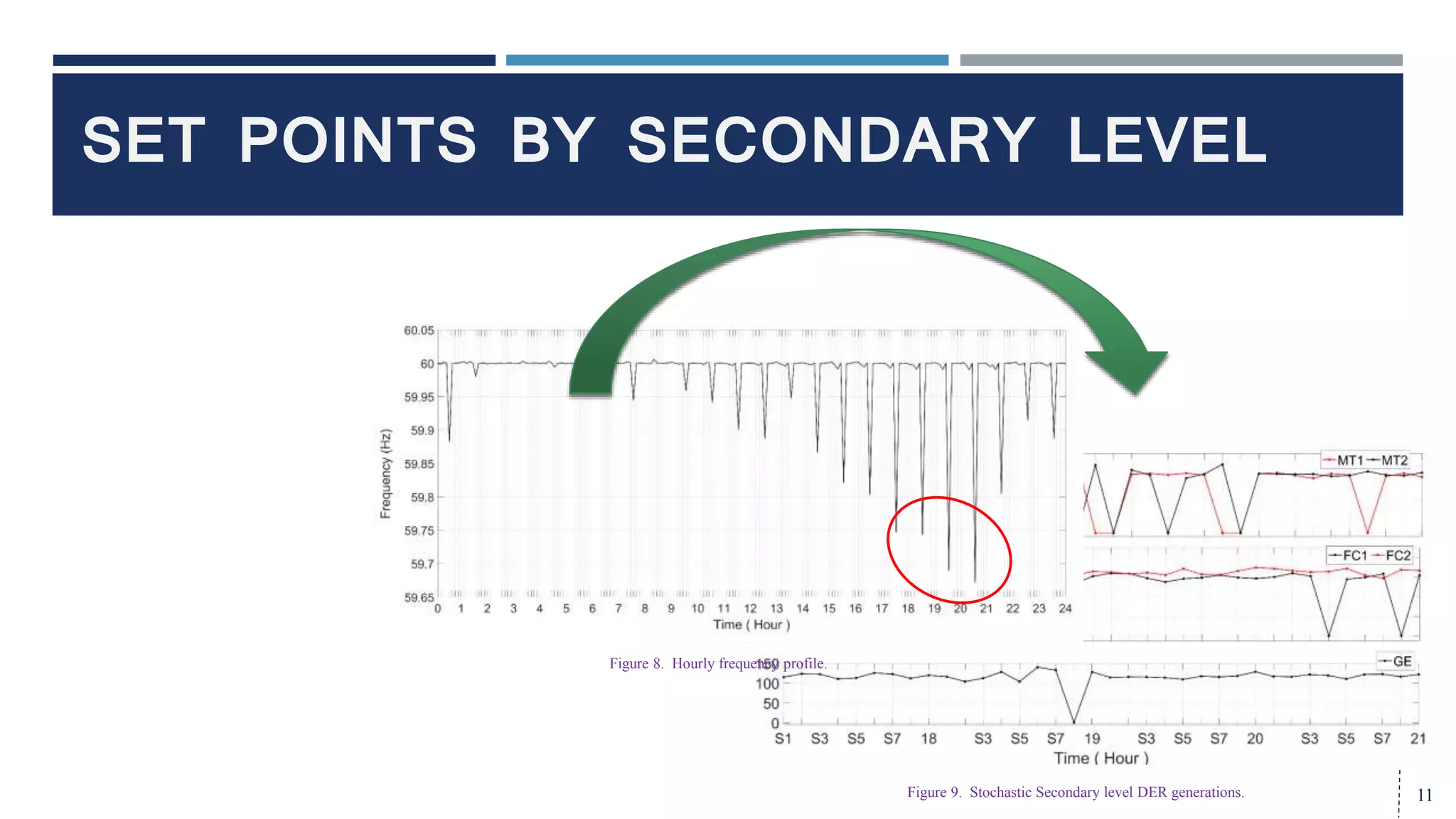
Hierarchical Droop Controlled Frequency Optimization and Energy Management of a Grid-Connected Microgrid , Sustech 2017 conference, Nov 12-14 Presented by Sima Aznavi

1. IEEE CONFERENCE ON TECHNOLOGIES FOR SUSTAINABILITY
Nov12-142017
By: Sima Aznavi, University of Nevada, Reno

2. CONTENTS
 Hierarchical Control
 Uncertainty Modeling
 Microgrid Test System
 Droop Control of DERs
 Objective Functions
 Total Emission
 Constraints
 Simulation Results
 Conclusions
2

3. Microgrid frequency
HIERARCHICAL CONTROL
 An efficient strategy for central energy management of the microgrid
1. Tertiary Control
 Distribution Network Operator (DNO) and Market Operator (MO) have main responsibilities
o such as management of importation/exportation of active and reactive power to/from the grid.
2. Secondary Control
 MGCC (Microgrid Central Controller)
 MGCC Task: Restoring the frequency and voltage of microgrid after disturbance
Changing the microgrid reference values and set points
Synchronizing with the grid
Optimizing operation of microgrid according to economic-environmental security goals
 Performances of the secondary and tertiary control level
o Interdependent and most of them are achieved by means of the MGCC
3. Primary Control
 Guarantees the fastest response to excursions, inner control of DERs to meet voltage/frequency reference set points.
3
𝑓 = 𝑓 𝑟𝑒𝑓 –
𝑚 𝑝 ( 𝑃𝑔 – 𝑃𝑟𝑒𝑓
)
Refer to the active power and
frequency reference set points
Active power
output of DERs
Droop coefficient for
each droop controller
 By applying the droop control method, microgrid voltage and frequency deviations from their corresponding
reference values can be regulated.
 The microgrid voltage and frequency deviations are regulated with respect to the reactive/active power
deviations: Key
player

4. UNCERTAINTY MODELING
4
1. Scenario Generation
2. Scenario Reduction
I. Latin Hypercube Sampling (LHS) is used to sample day-ahead load, wind and photovoltaic output forecast errors
II. Availability of DERs are modeled based on their Forced Outage Rates (FORs).
• The portion of time a unit is in demand, but is unavailable due to forced outages
1. A random number between 0 and 1 is generated for each scenario.
2. The random number is compared with the FOR.
FOR > Random Number ; DER : Out of service
else ; DER : Available2. Scenario Reduction
 considering a large number of scenarios increases the computational burden.
 Minimizing the number of generated scenarios without losing the generality of sampling.
 Scenarios’ probabilities < pre-specified value  Delete

5. Figure 1. Microgrid test system.
MICROGRID TEST SYSTEM
5
DER unit Pg
min (KW) Pg
max (KW) FOR E (Kg/KWh)
FC1 25 150 0.22 0.489
FC2 25 150 0.22 0.489
MT1 20 100 0.06 0.724
MT2 30 100 0.06 0.724
GE 35 200 0.02 0.85
TABLE I. Technical Data of The Microgrid Dispatchable DER Units
 Uncertainties in microgrid
load, wind turbine
generation, and photovoltaic
power output were
generated using the LHS
technique.
 Wi,h,s
DER is a randomly generated binary variable that shows the availability of the ith DER unit at hour h and in
scenario s.
 Wi,h,s
DER = 1 means that the ith DER unit is available in the hour h and scenario s
 Wi,h,s
DER = 0 expresses that the DER unit is out of service.
γ𝑖,ℎ,𝑠
𝐷𝐸𝑅
= W𝑖,ℎ,𝑠
𝐷𝐸𝑅
1 − FOR 𝑖
𝐷𝐸𝑅
+ 1 − W𝑖,ℎ,𝑠
𝐷𝐸𝑅
FOR 𝑖
𝐷𝐸𝑅
∗ W𝑖,ℎ−1,𝑠
𝐷𝐸𝑅
+ 1 − W𝑖,ℎ−1,𝑠
𝐷𝐸𝑅
Forced Outage Rate of the ith DER unit
Figure 2. Hourly forecasted vs. stochastic. wind turbine and photovoltaic power generation(Top) . load demand (Bottom).

6. Microgrid frequency deviation in
scenario s, control level m, and at hour h
DROOP CONTROL OF DERS
6
 P-f droop control technique applied to DERs by EMS
𝑖=1
𝑁 𝑔
∆𝑃𝑔( 𝑠, 𝑖, 𝑚, ℎ) = 𝑖=1
𝑁 𝑔
∆𝑃𝑟𝑒𝑓 𝑠, 𝑖, 𝑚, ℎ − 𝑖=1
𝑁 𝑔 1
𝑚 𝑝
∗ ∆𝑓 𝑠, 𝑚, ℎ , 𝑚 = 𝑝𝑟𝑖, 𝑠𝑒𝑐
Primary and Secondary
control levels
∆𝑃𝑔 𝑠, 𝑖, 𝑚, ℎ = 𝑃𝑔
𝑠 𝑖, 𝑚, ℎ − 𝑃𝑔 𝑖, ℎ
 Active power deviation of DER i
o in scenario s, control level m, and hour h.
𝑊𝑖,ℎ,𝑠
𝐷𝐸𝑅
∗
1
𝑚 𝑝 𝑖
∗ ∆𝑓 𝑠, 𝑚, ℎ = −𝑊𝑖,ℎ,𝑠
𝐷𝐸𝑅
∗ ∆𝑃𝑔 𝑠, 𝑖, 𝑚, ℎ , 𝑚 = 𝑝𝑟𝑖
𝑃𝑔
𝑠
𝑖, 𝑚, ℎ = 𝑊𝑖,ℎ,𝑠
𝐷𝐸𝑅
. 𝑃𝑟𝑒𝑓
𝑠
𝑖, 𝑚, ℎ −
1
𝑚 𝑝 𝑖
∗ ∆𝑓 𝑠, 𝑚, ℎ , 𝑚 = 𝑠𝑒𝑐
Active power output of DER i
in scenario s, control level m and hour h.
Forecasted active power output of DER i
at hour h.
∆𝑓 𝑠, 𝑝𝑟𝑖, ℎ =
− 𝑖=1
𝑁 𝑔
𝑊𝑖,ℎ,𝑠
𝐷𝐸𝑅
∗ ∆𝑃𝑔(𝑠, 𝑖, 𝑚, ℎ)
𝐷 𝑠, 𝑚, ℎ + 𝑖=1
𝑁 𝑔
𝑊𝑖,ℎ,𝑠
𝐷𝐸𝑅
∗
1
𝑚 𝑝(𝑖)
∆𝑓 𝑠, 𝑠𝑒𝑐, ℎ = 𝑖=1
𝑁 𝑔
𝑊𝑖,ℎ,𝑠
𝐷𝐸𝑅
∗ [𝑃𝑟𝑒𝑓
𝑠
𝑖, 𝑚, ℎ − 𝑃𝑔
𝑠
𝑖, 𝑚, ℎ ]
𝐷 𝑠, 𝑚, ℎ + 𝑖=1
𝑁 𝑔
𝑊𝑖,ℎ,𝑠
𝐷𝐸𝑅
∗
1
𝑚 𝑝(𝑖)
 In the primary level, reference power set point and the dispatched power output of the committed available
DER units are exactly equal, so: 𝑃𝑔
𝑠
𝑖, 𝑝𝑟𝑖, ℎ = 𝑃𝑟𝑒𝑓
𝑠
𝑖, 𝑝𝑟𝑖, ℎ
Reference power of DER i, in scenario s,
primary control level, and hour h

7.  This paper is dedicated to optimize steady state frequency deviation and
emissions considering technical constraints
 𝐹1 (ℎ) & 𝐹2 (ℎ) : objective functions
 Should be minimized in the multi-objective optimization
OBJECTIVE FUNCTIONS
7
𝐹1 ℎ =
𝑠=1
𝑁𝑠
𝜋 𝑠 ∗ |∆𝑓 𝑠, 𝑝𝑟𝑖, ℎ |
𝐹2(ℎ) = 𝐸(ℎ)

8. TOTAL EMISSION
8
𝐸 ℎ = 𝐸 𝑔𝑒𝑛 ℎ + 𝐸𝑟𝑒𝑑 ℎ
Hourly total generated emission Hourly total reduced emission
𝐸 𝑔𝑒𝑛 ℎ = 𝐸𝑔𝑟𝑖𝑑 ℎ + 𝑖=1
𝑁 𝑔
𝐸 𝑔(𝑖, ℎ) + 𝑠=1
𝑁𝑠
𝜋 𝑠 ( 𝑖=1
𝑁 𝑔
𝑚 𝐸 𝑔
𝑠
(𝑖, 𝑚, ℎ) + 𝑚 𝐸 𝑔𝑟𝑖𝑑
𝑠
𝑚, ℎ )
• Hourly generated emissions by utility grid
𝐸 𝑔𝑟𝑖𝑑 ℎ = 𝐸𝑔𝑟𝑖𝑑 ∗ 𝑃𝑔𝑟𝑖𝑑
ℎ , 𝐹𝑜𝑟 𝑃𝑔𝑟𝑖𝑑 ℎ > 0
Emission rates of utility grid
• Hourly generated emissions by the DERs
𝐸 𝑔(𝑖, ℎ) = 𝐸(𝑖) ∗ 𝑃𝑔
(𝑖, ℎ)
Emission rates of DER i
• Hourly generated emissions by DER i in scenario s
and control level m
𝐸 𝑔
𝑠(𝑖, 𝑚, ℎ) = 𝐸(𝑖) ∗ 𝑃𝑔
𝑠(𝑖, 𝑚, ℎ) 𝐸 𝑔𝑟𝑖𝑑
𝑠
𝑚, ℎ = 𝐸 𝑔𝑟𝑖𝑑 ∗ 𝑃𝑔𝑟𝑖𝑑
𝑠
𝑚, ℎ , 𝑃𝑔𝑟𝑖𝑑
𝑠
𝑚, ℎ > 0
• Hourly generated emissions by utility grid in
scenario s and control level m
When the excess power generated by the microgrid is sold back to the utility grid
𝑃𝑔𝑟𝑖𝑑 ℎ < 0
𝑃𝑔𝑟𝑖𝑑
𝑠
𝑚, ℎ < 0
𝐸𝑟𝑒𝑑 ℎ = 𝐸 𝑔_𝑟𝑒𝑑 ℎ +
𝑠=1
𝑁𝑠
𝜋 𝑠
𝑚
𝐸 𝑔_𝑟𝑒𝑑
𝑠
𝑚, ℎ ≤ 0
• Hourly reduced emissions by the DERs
𝐸 𝑔_𝑟𝑒𝑑 ℎ = 𝐸 𝑔𝑟𝑖𝑑 ∗ 𝑃𝑔𝑟𝑖𝑑
ℎ , 𝑃𝑔𝑟𝑖𝑑
ℎ < 0 𝐸 𝑔_𝑟𝑒𝑑
𝑠
𝑚, ℎ = 𝐸 𝑔𝑟𝑖𝑑 ∗ 𝑃𝑔𝑟𝑖𝑑
𝑠
𝑚, ℎ , 𝑃𝑔𝑟𝑖𝑑
𝑠
𝑚, ℎ < 0
• Hourly reduced emissions in scenario s and control level m

9. 𝐿𝑜𝑎𝑑 ℎ =
𝑖=1
𝑁 𝑔
𝑃𝑔 𝑖, ℎ +
𝑤=1
𝑁 𝑤
𝑃𝑤 𝑤, ℎ +
𝑣=1
𝑁 𝑣
𝑃𝑣 𝑣, ℎ + 𝑃𝑔𝑟𝑖𝑑 ℎ
CONSTRAINTS
9
 Power Balance
𝑖=1
𝑁 𝑔
𝑃𝑔
𝑠 𝑖, 𝑚, ℎ +
𝑤=1
𝑁 𝑤
𝑃𝑤
𝑠 𝑤, 𝑚, ℎ +
𝑣=1
𝑁 𝑣
𝑃𝑣
𝑠 𝑣, 𝑚, ℎ + 𝑃𝑔𝑟𝑖𝑑
𝑠
𝑚, ℎ = 𝐿𝑜𝑎𝑑 𝑠 𝑚, ℎ + 𝐷 𝑠, 𝑚, ℎ ∗ ∆𝑓 𝑠, 𝑚, ℎ
𝑃𝑔
𝑚𝑖𝑛(𝑖) ∗ 𝑊𝑖,ℎ,𝑠
𝐷𝐸𝑅
≤ 𝑃𝑔 𝑖, ℎ ≤ 𝑃𝑔
𝑚𝑎𝑥(𝑖) ∗ 𝑊𝑖,ℎ,𝑠
𝐷𝐸𝑅
𝑃𝑔
min
(𝑖) ∗ 𝑊𝑖,ℎ,𝑠
𝐷𝐸𝑅
≤ 𝑃𝑔
𝑠
𝑖, 𝑚, ℎ ≤ 𝑃𝑔
𝑚𝑎𝑥
(𝑖) ∗ 𝑊𝑖,ℎ,𝑠
𝐷𝐸𝑅

10. Figure 3. Hourly feasible pareto fronts.Figure 4. Optimum Droop Coefficients.
Figure 5. Hourly scheduled DER generations.
Figure 6. Stochastic Primary level DER generations.
Figure 7. Hourly power exchange with the grid.
SIMULATION RESULTS
10

11. SET POINTS BY SECONDARY LEVEL
11Figure 9. Stochastic Secondary level DER generations.
Figure 8. Hourly frequency profile.

12.  During intermittencies with sufficient droop controlled DERs, the primary control level is capable of mitigating the
frequency excursions in off-peak hours of the day
 No need for changes in the set points of the secondary control level in off-peak hours .
 During the peak hours the secondary control is required to change the set points of DERs.
 By increasing the penetration of droop controlled DERs in microgrid, the primary control level effectiveness in
providing the clean energy improves.
 The functionality of the proposed hierarchical Energy Management System in meeting the system security and
environmental concerns verifies the importance of droop controlled DERs in operational planning of the microgrid.
CONCLUSION
12
 Procedure:
1. A hierarchical Energy Management System in a typical grid-connected microgrid was presented.
2. The emphasis is on the droop controlled DERs as regulating units in primary frequency control during uncertainties.
3. An optimization scheme with objective functions of minimum frequency deviations and emissions is implemented.
4. A multi-objective approach to the Stochastic Fractal Search algorithm was applied to find the optimum solutions.
 Results :

13. QUESTIONS
13

14. Thank You
• Sima Aznavi
• s.aznavi@nevada.unr.edu
• (931) 529 - 1702