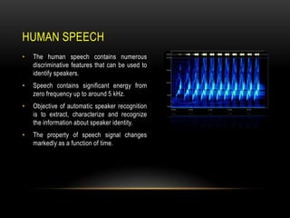
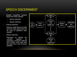
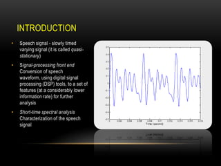
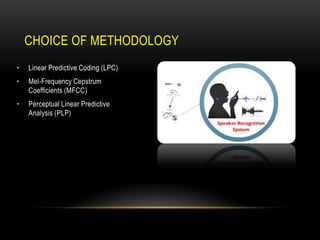
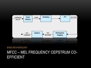
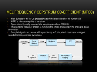
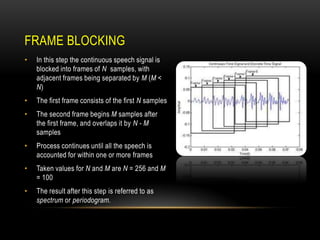
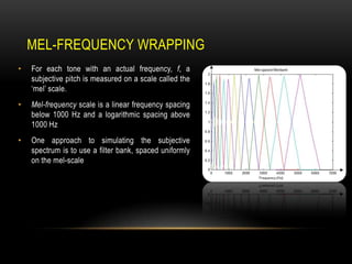
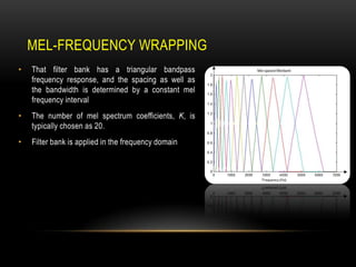
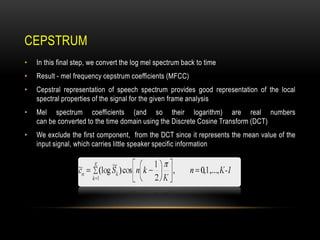
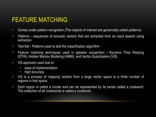
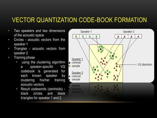
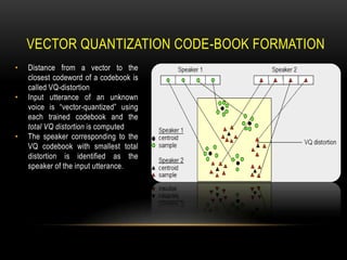
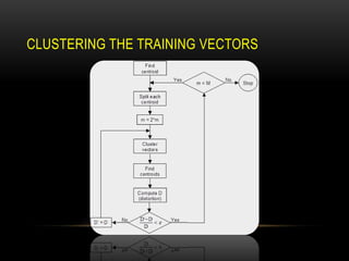
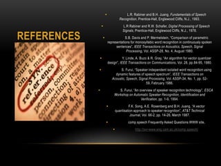
This document discusses speaker recognition using Mel Frequency Cepstral Coefficients (MFCC). It describes the process of feature extraction using MFCC which involves framing the speech signal, taking the Fourier transform of each frame, warping the frequencies using the mel scale, taking the logs of the powers at each mel frequency, and converting to cepstral coefficients. It then discusses feature matching techniques like vector quantization which clusters reference speaker features to create codebooks for comparison to unknown speakers. The document provides references for further reading on speech and speaker recognition techniques.

1. SPEAKER RECOGNITION USING MFCC
• Hira Shaukat 2010131
 DSP Lab Project
 Matlab-based programming
• Attiya Rehman 2010079

2. HUMAN SPEECH
•
The human speech contains numerous
discriminative features that can be used to
identify speakers.
•
Speech contains significant energy from
zero frequency up to around 5 kHz.
•
Objective of automatic speaker recognition
is to extract, characterize and recognize
the information about speaker identity.
•
The property of speech signal changes
markedly as a function of time.

3. SPEECH DISCERNMENT
•
Speaker recognition systems
contain two main modules:
•
•
•
feature extraction
feature matching
Feature extraction:
Extract a small amount of data
from the voice signal that can
be used to represent each
speaker
•
Feature matching:
Procedure to identify the
unknown
speaker
by
comparing extracted features
from his/her voice input with
the ones from a set of known
speakers

4. Phase 1
SPEECH FEATURE EXTRACTION

5. INTRODUCTION
•
Speech signal - slowly timed
varying signal (it is called quasistationary)
•
Signal-processing front end
Conversion of speech
waveform, using digital signal
processing (DSP) tools, to a set of
features (at a considerably lower
information rate) for further
analysis
•
Short-time spectral analysis
Characterization of the speech
signal

6. CHOICE OF METHODOLOGY
•
Linear Predictive Coding (LPC)
•
Mel-Frequency Cepstrum
Coefficients (MFCC)
•
Perceptual Linear Predictive
Analysis (PLP)

7. BASIC METHODOLOGY
MFCC – MEL FREQUENCY CEPSTRUM COEFFICIENT

8. MEL FREQUENCY CEPSTRUM CO-EFFICIENT (MFCC)
Main purpose of the MFCC processor is to mimic the behavior of the human ears
MFFC‟s - less susceptible to variations
Speech input typically recorded at a sampling rate above 10000 Hz
This sampling frequency chosen to minimize the effects of aliasing in the analog-to-digital
conversion
• Sampled signals can capture all frequencies up to 5 kHz, which cover most energy of
sounds that are generated by humans
•
•
•
•

9. FRAME BLOCKING
•
In this step the continuous speech signal is
blocked into frames of N samples, with
adjacent frames being separated by M (M <
N)
•
The first frame consists of the first N samples
•
The second frame begins M samples after
the first frame, and overlaps it by N - M
samples
•
Process continues until all the speech is
accounted for within one or more frames
•
Taken values for N and M are N = 256 and M
= 100
•
The result after this step is referred to as
spectrum or periodogram.

10. MEL-FREQUENCY WRAPPING
•
For each tone with an actual frequency, f, a
subjective pitch is measured on a scale called the
„mel‟ scale.
•
Mel-frequency scale is a linear frequency spacing
below 1000 Hz and a logarithmic spacing above
1000 Hz
•
One approach to simulating the subjective
spectrum is to use a filter bank, spaced uniformly
on the mel-scale

11. MEL-FREQUENCY WRAPPING
•
That filter bank has a triangular bandpass
frequency response, and the spacing as well as
the bandwidth is determined by a constant mel
frequency interval
•
The number of mel spectrum coefficients, K, is
typically chosen as 20.
•
Filter bank is applied in the frequency domain

12. CEPSTRUM
•
In this final step, we convert the log mel spectrum back to time
•
Result - mel frequency cepstrum coefficients (MFCC)
•
Cepstral representation of speech spectrum provides good representation of the local
spectral properties of the signal for the given frame analysis
•
Mel spectrum coefficients (and so their logarithm) are real numbers
can be converted to the time domain using the Discrete Cosine Transform (DCT)
•
We exclude the first component, from the DCT since it represents the mean value of the
input signal, which carries little speaker specific information

13. Phase 2
SPEECH FEATURE MATCHING

14. FEATURE MATCHING
•
Comes under pattern recognition (The objects of interest are generically called patterns)
•
Patterns - sequences of acoustic vectors that are extracted from an input speech using
extraction
•
Test Set - Patterns used to test the classification algorithm
•
Feature matching techniques used in speaker recognition - Dynamic Time Warping
(DTW), Hidden Markov Modeling (HMM), and Vector Quantization (VQ)
•
VQ approach used due to:
• ease of implementation
• high accuracy
VQ is a process of mapping vectors from a large vector space to a finite number of
regions in that space.
•
•
Each region is called a cluster and can be represented by its center called a codeword.
The collection of all codewords is called a codebook.

15. VECTOR QUANTIZATION CODE-BOOK FORMATION
•
•
•
•
Two speakers and two dimensions
of the acoustic space
Circles - acoustic vectors from the
speaker 1
Triangles - acoustic vectors from
speaker 2
Training phase
• using the clustering algorithm
a
speaker-specific
VQ
codebook is generated for
each known speaker by
clustering his/her training
acoustic vectors
• Result codewords (centroids) black circles and black
triangles for speaker 1 and 2

16. VECTOR QUANTIZATION CODE-BOOK FORMATION
•
•
•
Distance from a vector to the
closest codeword of a codebook is
called VQ-distortion
Input utterance of an unknown
voice is “vector-quantized” using
each trained codebook and the
total VQ distortion is computed
The speaker corresponding to the
VQ codebook with smallest total
distortion is identified as the
speaker of the input utterance.

17. CLUSTERING THE TRAINING VECTORS

18. Phase 3
MATLAB CODING

19. L.R. Rabiner and B.H. Juang, Fundamentals of Speech
Recognition, Prentice-Hall, Englewood Cliffs, N.J., 1993.

L.R Rabiner and R.W. Schafer, Digital Processing of Speech
Signals, Prentice-Hall, Englewood Cliffs, N.J., 1978.

REFERENCES

S.B. Davis and P. Mermelstein, “Comparison of parametric
representations for monosyllabic word recognition in continuously spoken
sentences”, IEEE Transactions on Acoustics, Speech, Signal
Processing, Vol. ASSP-28, No. 4, August 1980.

Y. Linde, A. Buzo & R. Gray, “An algorithm for vector quantizer
design”, IEEE Transactions on Communications, Vol. 28, pp.84-95, 1980.

S. Furui, “Speaker independent isolated word recognition using
dynamic features of speech spectrum”, IEEE Transactions on
Acoustic, Speech, Signal Processing, Vol. ASSP-34, No. 1, pp. 5259, February 1986.
S. Furui, “An overview of speaker recognition technology”, ESCA
Workshop on Automatic Speaker Recognition, Identification and
Verification, pp. 1-9, 1994.


F.K. Song, A.E. Rosenberg and B.H. Juang, “A vector
quantisation approach to speaker recognition”, AT&T Technical
Journal, Vol. 66-2, pp. 14-26, March 1987.

comp.speech Frequently Asked Questions WWW site,

http://svr-www.eng.cam.ac.uk/comp.speech/