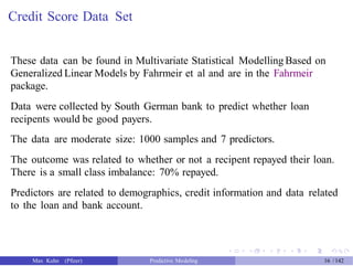
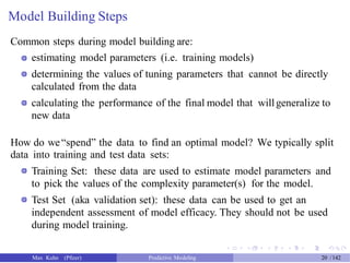
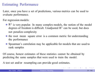
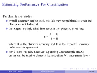
The document presents a comprehensive workshop on predictive modeling by Max Kuhn, covering essential concepts such as data types, modeling conventions in R, model building and evaluation, and various predictive modeling methods. It emphasizes the importance of splitting data for training and testing to avoid overfitting and discusses performance metrics for regression and classification models, including the use of ROC curves and confusion matrices. Additionally, it introduces the 'caret' package as a unified interface for modeling and streamlining processes in R.


![Credit Score Data Set
>
>
>
>
>
>
>
>
>
>
>
>
>
>
>
>
>
>
>
>
## translations, formatting, and dummy variables
library(Fahrmeir)
data(credit)
credit$Male <-ifelse(credit$Sexo == "hombre", 1, 0)
credit$Lives_Alone <-ifelse(credit$Estc == "vive solo", 1, 0)
credit$Good_Payer <-ifelse(credit$Ppag == "pre buen pagador", 1, 0)
credit$Private_Loan <-ifelse(credit$Uso == "privado", 1, 0)
credit$Class <-ifelse(credit$Y == "buen", "Good", "Bad")
credit$Class <- factor(credit$Class, levels = c("Good", "Bad"))
credit$Y <- NULL
credit$Sexo <- NULL
credit$Uso <- NULL
credit$Ppag <- NULL
credit$Estc <- NULL
names(credit)[names(credit) == "Mes"] <- "Loan_Duration"
names(credit)[names(credit) == "DM"] <- "Loan_Amount"
names(credit)[names(credit) == "Cuenta"] <- "Credit_Quality"
Max Kuhn (Pfizer) Predictive Modeling 17 /142](https://image.slidesharecdn.com/maxkuhnpredictivemodelingworkshop-150603155123-lva1-app6891/85/Predictive-Modeling-Workshop-18-320.jpg)


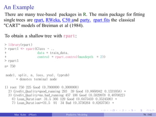
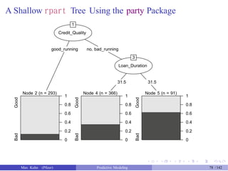
![Credit Data Set
For these data, let’s take a stratified random sample of 760 loans for
training.
> set.seed(8140)
> in_train <- createDataPartition(credit$Class, p = .75, list = FALSE)
> head(in_train)
Resample1
[1,]
[2,]
[3,]
[4,]
[5,]
[6,]
1
2
3
4
5
8
> train_data <- credit[ in_train,]
> test_data <- credit[-in_train,]
Max Kuhn (Pfizer) Predictive Modeling 23 /142](https://image.slidesharecdn.com/maxkuhnpredictivemodelingworkshop-150603155123-lva1-app6891/85/Predictive-Modeling-Workshop-24-320.jpg)


![Dummy Variables
> alt_data <- model.matrix(Class ~ ., data = train_data)
> alt_data[1:4, 1:3]
(Intercept) Credit_Qualitygood_running Credit_Qualitybad_running
1
2
3
4
1
1
1
1
0
0
0
0
0
0
1
0
We can get rid of the intercept column and use this data.
However, we would want to apply this same transformation to new data
sets.
The caret function dummyVars has more options and can be applied to any
data
Note: using the formula method with models automatically handles this.
Max Kuhn (Pfizer) Predictive Modeling 51 /142](https://image.slidesharecdn.com/maxkuhnpredictivemodelingworkshop-150603155123-lva1-app6891/85/Predictive-Modeling-Workshop-52-320.jpg)
![Dummy Variables
> dummy_info <- dummyVars(Class ~ ., data = train_data)
> dummy_info
Dummy Variable Object
Formula: Class ~ .
8 variables, 2 factors
Variables and levels will be separated by '.'
A less than full rank encoding is used
> train_dummies <- predict(dummy_info, newdata = train_data)
> train_dummies[1:4, 1:3]
Credit_Quality.no Credit_Quality.good_running Credit_Quality.bad_running
1
2
3
4
1
1
0
1
0
0
0
0
0
0
1
0
> test_dummies <- predict(dummy_info, newdata = test_data)
Max Kuhn (Pfizer) Predictive Modeling 52 /142](https://image.slidesharecdn.com/maxkuhnpredictivemodelingworkshop-150603155123-lva1-app6891/85/Predictive-Modeling-Workshop-53-320.jpg)


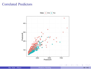
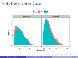
![An Example
Another data set shows an nice example of PCA. There are two the
predictors and two classes:
> dim(example_train)
[1] 1009 3
> dim(example_test)
[1] 1010 3
> head(example_train)
PredictorA PredictorB Class
2
3
4
12
15
16
3278.726
1727.410
1194.932
1027.222
1035.608
1433.918
154.89876
84.56460
101.09107
68.71062
73.40559
79.47569
One
Two
One
Two
One
One
Max Kuhn (Pfizer) Predictive Modeling 59 /142](https://image.slidesharecdn.com/maxkuhnpredictivemodelingworkshop-150603155123-lva1-app6891/85/Predictive-Modeling-Workshop-60-320.jpg)
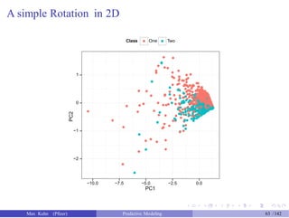
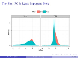
![An Example
> pca_pp <- preProcess(example_train[, 1:2],
+
> pca_pp
method = "pca") # also added "center" and "scale"
Call:
preProcess.default(x = example_train[, 1:2], method = "pca")
Created from 1009 samples and 2 variables
Pre-processing: principal component signal extraction, scaled, centered
PCA needed 2 components to capture 95 percent of the variance
> train_pc <- predict(pca_pp, example_train[, 1:2])
> test_pc <- predict(pca_pp, example_test[, 1:2])
> head(test_pc, 4)
PC1
1 0.8420447
5 0.2189168
6 1.2074404
PC2
0.07284802
0.04568417
-0.21040558
7 1.1794578 -0.20980371
Max Kuhn (Pfizer) Predictive Modeling 62 /142](https://image.slidesharecdn.com/maxkuhnpredictivemodelingworkshop-150603155123-lva1-app6891/85/Predictive-Modeling-Workshop-63-320.jpg)

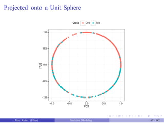
![Adding Another Step
> pca_ss_pp <- preProcess(example_train[, 1:2],
+
> pca_ss_pp
method = c("pca", "spatialSign"))
Call:
preProcess.default(x = example_train[, 1:2], method = c("pca", "spatialSign"))
Created from 1009 samples and 2 variables
Pre-processing: principal component signal extraction, spatial
sign transformation, scaled, centered
PCA needed 2 components to capture 95 percent of the variance
> train_pc_ss <- predict(pca_ss_pp, example_train[, 1:2])
> test_pc_ss <- predict(pca_ss_pp, example_test[, 1:2])
> head(test_pc_ss, 4)
PC1
1 0.9962786
5 0.9789121
6 0.9851544
PC2
0.08619129
0.20428207
-0.17167058
7 0.9845449 -0.17513231
Max Kuhn (Pfizer) Predictive Modeling 66 /142](https://image.slidesharecdn.com/maxkuhnpredictivemodelingworkshop-150603155123-lva1-app6891/85/Predictive-Modeling-Workshop-67-320.jpg)


![Example: Encoding Time and Date Data
I have found the lubridate package to be invaluable in these cases.
Let’s load some example dates from an existing RData file:
> day_values <- c("2015-05-10", "1970-11-04", "2002-03-04", "2006-01-13")
> class(day_values)
[1] "character"
> library(lubridate)
> days <- ymd(day_values)
> str(days)
POSIXct[1:4], format: "2015-05-10" "1970-11-04" "2002-03-04" "2006-01-13"
Max Kuhn (Pfizer) Predictive Modeling 72 /142](https://image.slidesharecdn.com/maxkuhnpredictivemodelingworkshop-150603155123-lva1-app6891/85/Predictive-Modeling-Workshop-73-320.jpg)
![Example: Encoding Time and Date Data
> day_of_week <- wday(days, label = TRUE)
> day_of_week
[1] Sun Wed Mon Fri
Levels: Sun < Mon < Tues < Wed < Thurs < Fri < Sat
> year(days)
[1] 2015 1970 2002 2006
> week(days)
[1] 19 45 10 2
> month(days, label = TRUE)
[1] May Nov Mar Jan
12 Levels: Jan < Feb < Mar < Apr < May < Jun < Jul < Aug < Sep < ... < Dec
> yday(days)
[1] 130 308 63 13
Max Kuhn (Pfizer) Predictive Modeling 73 /142](https://image.slidesharecdn.com/maxkuhnpredictivemodelingworkshop-150603155123-lva1-app6891/85/Predictive-Modeling-Workshop-74-320.jpg)


![Test Set Results
> rpart_pred <- predict(rpart_full, newdata = test_data, type = "class")
> confusionMatrix(data = rpart_pred, reference = test_data$Class)
Confusion Matrix and Statistics
# requires 2 factor vectors
Reference
Prediction Good Bad
Good 163 49
Bad 12 26
Accuracy : 0.756
95% CI : (0.6979, 0.8079)
No Information Rate : 0.7
P-Value [Acc > NIR] : 0.02945
Kappa : 0.3237
Mcnemar's Test P-Value : 4.04e-06
Sensitivity : 0.9314
Specificity : 0.3467
Pos Pred Value : 0.7689
Neg Pred Value : 0.6842
Prevalence : 0.7000
Detection Rate : 0.6520
Detection Prevalence : 0.8480
Balanced Accuracy : 0.6390
'Positive' Class : Good
Max Kuhn (Pfizer) Predictive Modeling 83 /142](https://image.slidesharecdn.com/maxkuhnpredictivemodelingworkshop-150603155123-lva1-app6891/85/Predictive-Modeling-Workshop-84-320.jpg)
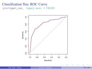
![Creating the ROC Curve
The pROC package can be used to create ROC curves.
The function roc is used to capture the data and compute the ROC curve.
The functions plot.roc and auc.roc generate plot and area under the
curve, respectively.
> class_probs <- predict(rpart_full, newdata = test_data)
> head(class_probs, 3)
Good Bad
6 0.8636364 0.1363636
7 0.8636364 0.1363636
13 0.8636364 0.1363636
> library(pROC)
> ## The roc function assumes the *second* level is the one of
> ## interest, so we use the 'levels' argument to change the order.
> rpart_roc <- roc(response = test_data$Class, predictor = class_probs[, "Good"],
+ levels = rev(levels(test_data$Class)))
> ## Get the area under the ROC curve
> auc(rpart_roc)
Area under the curve: 0.7975
Max Kuhn (Pfizer) Predictive Modeling 84 /142](https://image.slidesharecdn.com/maxkuhnpredictivemodelingworkshop-150603155123-lva1-app6891/85/Predictive-Modeling-Workshop-85-320.jpg)


![Test Set Results
> rpart_pred2 <- predict(rpart_tune, newdata = test_data)
> confusionMatrix(rpart_pred2, test_data$Class)
Confusion Matrix and Statistics
Reference
Prediction Good Bad
Good 161 47
Bad 14 28
Accuracy : 0.756
95% CI : (0.6979, 0.8079)
No Information Rate : 0.7
P-Value [Acc > NIR] : 0.02945
Kappa : 0.3355
Mcnemar's Test P-Value : 4.182e-05
Sensitivity : 0.9200
Specificity : 0.3733
Pos Pred Value : 0.7740
Neg Pred Value : 0.6667
Prevalence : 0.7000
Detection Rate : 0.6440
Detection Prevalence : 0.8320
Balanced Accuracy : 0.6467
'Positive' Class : Good
Max Kuhn (Pfizer) Predictive Modeling 100 /142](https://image.slidesharecdn.com/maxkuhnpredictivemodelingworkshop-150603155123-lva1-app6891/85/Predictive-Modeling-Workshop-101-320.jpg)
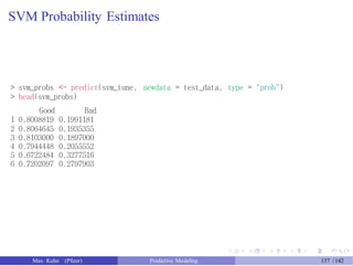
![Predicting Class Probabilities
predict.train has an argument type that can be used to get predicted
class probabilities for different models:
> rpart_probs <- predict(rpart_tune, newdata = test_data, type = "prob")
> head(rpart_probs, n = 4)
Good Bad
6 0.8636364 0.1363636
7 0.8636364 0.1363636
13 0.8636364 0.1363636
16 0.8636364 0.1363636
> rpart_roc <- roc(response = test_data$Class, predictor = rpart_probs[, "Good"],
+
> auc(rpart_roc)
levels = rev(levels(test_data$Class)))
Area under the curve: 0.8154
Max Kuhn (Pfizer) Predictive Modeling 101 /142](https://image.slidesharecdn.com/maxkuhnpredictivemodelingworkshop-150603155123-lva1-app6891/85/Predictive-Modeling-Workshop-102-320.jpg)


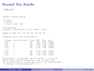
![gbm Predictions
We need to tell the predict method how many trees to use (let’s just pick
500).
Also, it does not predict the actual class. We’ll get the class probability
and do the conversion.
> gbm_pred <- predict(gbm_fit, newdata = test_data, n.trees = 100,
+
+
> head(gbm_pred)
## This calculates the class probs
type = "response")
[1] 0.6803420 0.7628453 0.6882552 0.8262940 0.8861083 0.7280930
> gbm_pred <- factor(ifelse(gbm_pred > .5, "Good", "Bad"),
+
> head(gbm_pred)
levels = c("Good", "Bad"))
[1] Good Good Good Good Good Good
Levels: Good Bad
Max Kuhn (Pfizer) Predictive Modeling 110 /142](https://image.slidesharecdn.com/maxkuhnpredictivemodelingworkshop-150603155123-lva1-app6891/85/Predictive-Modeling-Workshop-111-320.jpg)
![Test Set Results
> confusionMatrix(gbm_pred, test_data$Class)
Confusion Matrix and Statistics
Reference
Prediction Good Bad
Good 166 51
Bad 9 24
Accuracy : 0.76
95% CI : (0.7021, 0.8116)
No Information Rate : 0.7
P-Value [Acc > NIR] : 0.02104
Kappa : 0.3197
Mcnemar's Test P-Value : 1.203e-07
Sensitivity : 0.9486
Specificity : 0.3200
Pos Pred Value : 0.7650
Neg Pred Value : 0.7273
Prevalence : 0.7000
Detection Rate : 0.6640
Detection Prevalence : 0.8680
Balanced Accuracy : 0.6343
'Positive' Class : Good
Max Kuhn (Pfizer) Predictive Modeling 111 /142](https://image.slidesharecdn.com/maxkuhnpredictivemodelingworkshop-150603155123-lva1-app6891/85/Predictive-Modeling-Workshop-112-320.jpg)

![Another Digression – The Ellipses
R has a great feature known as the ellipses(aka "three dots") where an
arbitrary number of function arguments can be pass through nested
function calls. For example:
> average <- function(dat, ...) mean(dat, ...)
> names(formals(mean.default))
[1] "x" "trim" "na.rm" "..."
> average(dat = c(1:10, 100))
[1] 14.09091
> average(dat = c(1:10, 100), trim = .1)
[1] 6
train is structured to take full advantage of this so that arguments can
be passed to the underlying model function (e.g. rpart, gbm) when calling
the train function.
Max Kuhn (Pfizer) Predictive Modeling 113 /142](https://image.slidesharecdn.com/maxkuhnpredictivemodelingworkshop-150603155123-lva1-app6891/85/Predictive-Modeling-Workshop-114-320.jpg)

![Test Set Results
> gbm_pred <- predict(gbm_tune, newdata = test_data) # Magic!
> confusionMatrix(gbm_pred, test_data$Class)
Confusion Matrix and Statistics
Reference
Prediction Good Bad
Good 167 52
Bad 8 23
Accuracy : 0.76
95% CI : (0.7021, 0.8116)
No Information Rate : 0.7
P-Value [Acc > NIR] : 0.02104
Kappa : 0.3135
Mcnemar's Test P-Value : 2.836e-08
Sensitivity : 0.9543
Specificity : 0.3067
Pos Pred Value : 0.7626
Neg Pred Value : 0.7419
Prevalence : 0.7000
Detection Rate : 0.6680
Detection Prevalence : 0.8760
Balanced Accuracy : 0.6305
'Positive' Class : Good
Max Kuhn (Pfizer) Predictive Modeling 117 /142](https://image.slidesharecdn.com/maxkuhnpredictivemodelingworkshop-150603155123-lva1-app6891/85/Predictive-Modeling-Workshop-118-320.jpg)

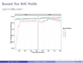
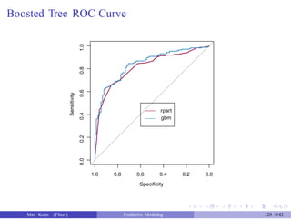
![Boosted Tree ROC Curve
> gbm_roc <- roc(response = test_data$Class, predictor = gbm_probs[, "Good"],
+
> auc(rpart_roc)
levels = rev(levels(test_data$Class)))
Area under the curve: 0.8154
> auc(gbm_roc)
Area under the curve: 0.8422
> plot(rpart_roc, col = "#9E0142", legacy.axes = FALSE)
> plot(gbm_roc, col = "#3288BD", legacy.axes = FALSE, add = TRUE)
> legend(.6, .5, legend = c("rpart", "gbm"),
+
+
lty = c(1, 1),
col = c("#9E0142", "#3288BD"))
Max Kuhn (Pfizer) Predictive Modeling 119 /142](https://image.slidesharecdn.com/maxkuhnpredictivemodelingworkshop-150603155123-lva1-app6891/85/Predictive-Modeling-Workshop-120-320.jpg)


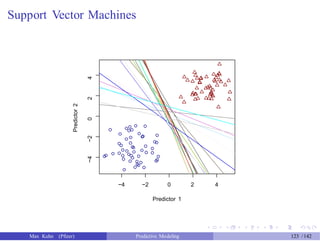

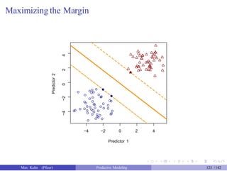


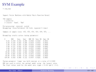
![Tuning SVM Models
We need to come up with reasonable choices for the cost parameter and
any other parameters associated with the kernel, such as
polynomial degree for the polynomial kernel
a, the scale parameter for radial basis functions (RBF)
We’ll focus on RBF kernel models here, so we have two tuning parameters.
However, there is a potential shortcut for RBF kernels. Reasonable values
of a can be derived from elements of the kernel matrix of the training set.
The manual for the sigest function in kernlab has "The estimation [for a]
is based upon the 0.1 and 0.9 quantile of lx - x tl2."
Anecdotally, we have found that the mid-point between these two
numbers can provide a good estimate for this tuning parameter. This
leaves only the cost function for tuning.
Max Kuhn (Pfizer) Predictive Modeling 131 /142](https://image.slidesharecdn.com/maxkuhnpredictivemodelingworkshop-150603155123-lva1-app6891/85/Predictive-Modeling-Workshop-132-320.jpg)


![Test Set Results
> svm_pred <- predict(svm_tune, newdata = test_data)
> confusionMatrix(svm_pred, test_data$Class)
Confusion Matrix and Statistics
Reference
Prediction Good Bad
Good 165 49
Bad 10 26
Accuracy : 0.764
95% CI : (0.7064, 0.8152)
No Information Rate : 0.7
P-Value [Acc > NIR] : 0.01474
Kappa : 0.34
Mcnemar's Test P-Value : 7.53e-07
Sensitivity : 0.9429
Specificity : 0.3467
Pos Pred Value : 0.7710
Neg Pred Value : 0.7222
Prevalence : 0.7000
Detection Rate : 0.6600
Detection Prevalence : 0.8560
Balanced Accuracy : 0.6448
'Positive' Class : Good
Max Kuhn (Pfizer) Predictive Modeling 136 /142](https://image.slidesharecdn.com/maxkuhnpredictivemodelingworkshop-150603155123-lva1-app6891/85/Predictive-Modeling-Workshop-137-320.jpg)
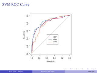
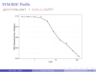
![SVM ROC Curve
> svm_roc <- roc(response = test_data$Class, predictor = svm_probs[, "Good"],
+
> auc(rpart_roc)
levels = rev(levels(test_data$Class)))
Area under the curve: 0.8154
> auc(gbm_roc)
Area under the curve: 0.8422
> auc(svm_roc)
Area under the curve: 0.7838
> plot(rpart_roc, col = "#9E0142", legacy.axes = FALSE)
> plot(gbm_roc, col = "#3288BD", legacy.axes = FALSE, add = TRUE)
> plot(svm_roc, col = "#F46D43", legacy.axes = FALSE, add = TRUE)
> legend(.6, .5, legend = c("rpart", "gbm", "svm"),
+
+
lty = c(1, 1, 1),
col = c("#9E0142", "#3288BD", "#F46D43"))
Max Kuhn (Pfizer) Predictive Modeling 138 /142](https://image.slidesharecdn.com/maxkuhnpredictivemodelingworkshop-150603155123-lva1-app6891/85/Predictive-Modeling-Workshop-139-320.jpg)