Download as PDF, PPTX


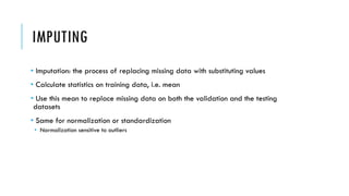
![R EXAMPLE
k = 5
results <- numeric(k)
ind <- sample(2, nrow(iris), replace=T, prob=c(0.8, 0.2))
trainval <- iris[ind==1,]
test <- iris[ind !=1,]
cv <- sample(rep(1:k, length.out=nrow(trainval)))
for(i in 1:k) {
trainData <- trainval[cv != i,]
valData <- trainval[cv == i,]
model <- naiveBayes(Species ~ ., data=trainData, laplace = 0)
pred <- predict(model, valData)
results[i] <- Accuracy(pred, valData$Species)
}
print(mean(results))
# after finding the best laplace
finalmodel <- naiveBayes(Species ~ ., data=trainval,
laplace = 0)
pred <- predict(finalmodel, test)
print(Accuracy(pred, test$Species))
Validation - 0.95 vs. 0.91 - Test](https://image.slidesharecdn.com/ece-ama-ml-190521072126/85/Simple-rules-for-building-robust-machine-learning-models-11-320.jpg)


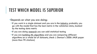
![BOX-PLOTS
g <- list()
j <- 1
long <- melt(data)
for(i in names(data)) {
subdata = long[long$variable == i,]
g[[j]] <- ggplot(data = subdata,
aes(x=variable, y=value)) +
geom_boxplot()
j = j+1
}
grid.arrange(grobs=g, nrow = 2)
- Check outliers](https://image.slidesharecdn.com/ece-ama-ml-190521072126/85/Simple-rules-for-building-robust-machine-learning-models-26-320.jpg)
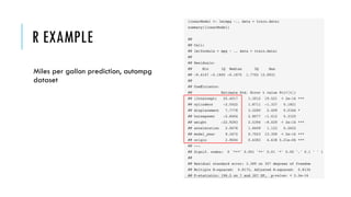
![DENSITY PLOTS
g <- list()
j <- 1
for(i in names(data)) {
print(i)
p <- ggplot(data = data,
aes_string(x=i)) +
geom_density()
g[[j]] <- p
j = j+1
}
grid.arrange(grobs=g, nrow = 2)
- Check normally distributed or right/positively skewed](https://image.slidesharecdn.com/ece-ama-ml-190521072126/85/Simple-rules-for-building-robust-machine-learning-models-27-320.jpg)

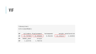
![PROPROCESSING
EXAMPLES IN R
ind <- sample(3, nrow(data), replace=TRUE,
prob=c(0.6, 0.2, 0.2))
trainData <- data[ind==1,]
valData <- data[ind==2,]
testData <- data[ind==3,]
trainMaxs <- apply(trainData[,1:11], 2, max)
trainMins <- apply(trainData[,1:11], 2, min)
normTrainData <-
sweep(sweep(trainData[,1:11], 2, trainMins, "-"),
2, (trainMaxs - trainMins), "/")
summary(normTrainData)](https://image.slidesharecdn.com/ece-ama-ml-190521072126/85/Simple-rules-for-building-robust-machine-learning-models-30-320.jpg)
![PROPROCESSING
EXAMPLES IN R
normValData <- sweep(sweep(valData[,1:11],
2, trainMins, "-"), 2, (trainMaxs - trainMins), "/")
Not an issue if data is big and
correct sampling is kept.](https://image.slidesharecdn.com/ece-ama-ml-190521072126/85/Simple-rules-for-building-robust-machine-learning-models-31-320.jpg)


![EXAMPLE IN R
results <- numeric(100)
for(i in 1:100) {
ind <- sample(2, nrow(iris), replace=T,
prob=c(0.9, 0.1))
trainData <- iris[ind==1,]
valData <- iris[ind==2,]
model <- naiveBayes(Species ~ .,
data=trainData)
pred <- predict(model, valData)
results[i] <- Accuracy(pred,
valData$Species)
}
• Even in this simple dataset and
scenario….55/100 splits gave perfect score
in one run.
• With simple 10-fold cross-validation I could
have gotten 100% validation accuracy.
• In one run I got 70%...30% difference
based on luck.](https://image.slidesharecdn.com/ece-ama-ml-190521072126/85/Simple-rules-for-building-robust-machine-learning-models-34-320.jpg)


![R EXAMPLEresultsMA <- numeric(10)
resultsMB <- numeric(10)
cv <- sample(rep(1:10, nrow(iris)/10))
for(i in 1:10) {
trainData <- iris[cv == i,]
valData <- iris[cv != i,]
model <- naiveBayes(Species ~ ., data=trainData)
pred <- predict(model, valData)
resultsMA[i] <- Accuracy(pred, valData$Species)
ctree = rpart(Species ~ ., data=trainData,
method="class",minsplit = 1, minbucket = 1, cp = -1)
pred <- predict(ctree, valData, type="class")
resultsMB[i] <- Accuracy(pred, valData$Species)
}
wilcoxon.test(resultsMA, resultsMB)
If p value less than confidence level
then there is statistical significance.](https://image.slidesharecdn.com/ece-ama-ml-190521072126/85/Simple-rules-for-building-robust-machine-learning-models-38-320.jpg)


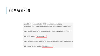


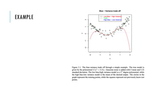


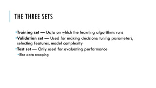
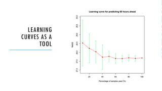
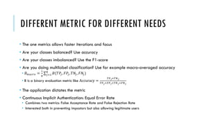
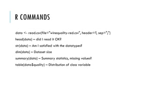
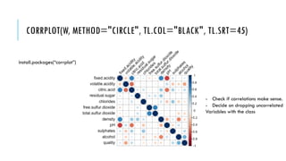
The document outlines simple rules for building robust machine learning models, emphasizing the importance of splitting data into training, validation, and test sets, and ensuring each set is representative of future data distributions. It discusses various metrics for model evaluation, the significance of exploratory data analysis, and the impact of data preprocessing on model performance. Additionally, it covers guidelines for selecting appropriate algorithms, tuning hyperparameters, and conducting experiments efficiently.