- The document describes a machine learning project that analyzed data from wearable sensors to predict the manner in which exercises were performed.
- The author tested decision trees, random forests, and boosted regressions on the data, and found that random forests had the lowest error rate at 0.06%. Random forests was thus used as the optimal predictive model.
This document showcases the work of Qanka Studio, an design studio. It includes brief descriptions and images for over 15 projects spanning various types of design work like publication design, user interface design, branding, identity design, and communication design. The projects cover diverse clients and industries like education, fashion, hospitality, and non-profits. It concludes by thanking the viewer and providing the studio's contact information.
1. The document provides instructions for using Dropbox to store and share files across devices. It explains how to install Dropbox on computers and mobile devices, upload and access files from any device, and share files and folders with others by generating links or setting up shared folders.
2. Dropbox allows users to automatically backup files to the cloud so they are safe if a device is lost or broken. Installed on multiple devices, it syncs files across all devices so users always have access to their latest files anywhere.
3. The instructions also cover sending large files through shared links, collaborating with others in real-time by creating shared folders, and additional security and premium features through Dropbox Pro and for Business.
El documento habla sobre el aprendizaje autónomo. Explica que los estilos y resultados de aprendizaje varían entre personas y situaciones. También menciona que todos pueden desarrollar cierta capacidad para la autodirección en el aprendizaje. Además, señala que la autonomía no significa aislamiento sino que requiere organización del tiempo y recursos.
The document is a job description for a Facilities Maintenance Technician position with the San Mateo Union High School District. The job involves performing repairs and maintenance on HVAC, plumbing, and other mechanical systems. Duties include inspecting and servicing boiler, ventilation, and refrigeration equipment; estimating costs for repairs; and completing paperwork to ensure compliance. Qualifications include a high school diploma, apprenticeship completion, journey-level experience, and licenses/certifications in HVAC-R and refrigerants. The position requires working both indoors and outdoors, with hazards like fumes, moving machinery, and heights.
- In 3Q 2015, NOL reported a net loss of $96 million and core EBIT loss of $66 million due to weak freight rates and volumes across all trades. YTD 2015 net profit was $783 million including a one-time gain on sale of APL Logistics.
- Freight rates declined 28-48% YoY in 3Q 2015 due to overcapacity and weak trade growth. Volume and revenue per FEU also decreased YoY.
- NOL achieved $80 million in cost savings in 3Q 2015 through network optimization, charter expiries and other measures, partially offsetting declines. Further cost reductions are planned in 4Q 2015.
The document discusses lions and efforts to save them from extinction. It notes that lions are currently the second largest big cat species and live in prides led by males. While lions originally inhabited parts of Africa, Asia, and Europe, their population has declined 43% and they are now endangered. Some ways to help save lions discussed are increasing awareness, strengthening laws against poaching, protecting habitats, and effectively managing wildlife refuge systems.
This document downloads training and testing data files for a machine learning model. It then cleans the training data, removing columns with missing or non-numeric values. A random forest model is trained on 70% of the cleaned training data and predicts classes for the remaining 30%, achieving 99.4% accuracy based on a confusion matrix. The trained model is then used to predict classes for the cleaned testing data.
The document describes a machine learning project to classify different types of bicep curl exercises using sensor data from wearable devices. A random forest model was trained on 53 variables from the sensor data to classify exercises into 5 categories with high accuracy (>99%). Variable importance analysis showed that variables related to arm movement and acceleration were most important for classification. The model was tested on held-out data and achieved similar high accuracy, demonstrating the model's ability to generalize.
Construire un modèle prédictif avec TensorflowEric Bustarret
This document summarizes the steps to build a predictive model with TensorFlow. It discusses collecting data, preparing the dataset by separating features and labels, scaling features, and splitting data into training and test sets. It describes selecting a neural network model with one hidden layer and training it. Model performance is evaluated using metrics like confusion matrix and classification report. Tuning hyperparameters like the number of hidden layers and neurons can help avoid underfitting or overfitting. The model can then be deployed once validated.
Data science with R - Clustering and ClassificationBrigitte Mueller
This presentation guides you through your first steps to a prediction with R. We predict flight delays using classification. I prepared and cleaned the data and split them into train and test data (github link /mbbrigitte).
The talk was held in May 2016 for Ruby programmers.
1. A random forest model achieved over 90% accuracy on the training data but had some errors predicting classes for the testing data.
2. Most prediction errors occurred near the centers of each class, possibly due to overfitting, and reducing features could help.
3. The graphs show some classes (A, B, C, D) were sometimes confused with each other, likely because small form errors could cause assignment to different classes.
Forecasting Revenue With Stationary Time Series ModelsGeoffery Mullings
A trend stationary time series model was used to forecast Starbucks' quarterly revenue over multiple quarters into the future based on historical data. The model predicted 2015 Q4 revenue within 0.33 standard deviations of the actual reported revenue and correctly predicted an increase in the short-term. Logarithmic transformation of the revenue values helped linearize the model. Statistical analysis identified revenue in the prior quarter, and the first and second lags of revenue changes as significant predictors of future revenue changes.
Building ML Pipelines:
- What do ML Pipelines Look Like?
- Building one ML pipeline
- ML pipeline in code
- Why use ML pipeline?
By Debidatta Dwibedi, presented at Data Science Meetup at InMobi.
http://technology.inmobi.com/events/data-science-meetup
This document discusses machine learning pipelines. It explains that ML pipelines involve multiple steps like data preprocessing, feature extraction, training models with different hyperparameters, and testing models. The goal is to build the best model by evaluating many variations systematically. Key steps are often cross-validation to evaluate models and hyperparameter tuning to find the best configuration. Well-designed ML pipelines can help improve model performance and make the process more efficient and reproducible.
These are the slides from workshop: Introduction to Machine Learning with R which I gave at the University of Heidelberg, Germany on June 28th 2018.
The accompanying code to generate all plots in these slides (plus additional code) can be found on my blog: https://shirinsplayground.netlify.com/2018/06/intro_to_ml_workshop_heidelberg/
The workshop covered the basics of machine learning. With an example dataset I went through a standard machine learning workflow in R with the packages caret and h2o:
- reading in data
- exploratory data analysis
- missingness
- feature engineering
- training and test split
- model training with Random Forests, Gradient Boosting, Neural Nets, etc.
- hyperparameter tuning
The document describes downloading and processing the Reuters news dataset to create training and test datasets for text classification. Key steps include:
1. Downloading the Reuters dataset and processing it to create feature vectors (x_train, x_test) and labels (y_train, y_test).
2. Creating a simple neural network model with an input, two hidden layers and an output layer.
3. Training the model on the training data for 20 epochs and evaluating performance on the validation set, showing decreasing loss and increasing accuracy over epochs.
Dimensionality reduction, or dimension reduction, is the transformation of data from a high-dimensional space into a low-dimensional space so that the low-dimensional representation retains some meaningful properties of the original data
The document compares the performance of four common data mining algorithms (KNN, decision trees, EM, and k-means clustering) across three datasets. It describes the datasets, experimental procedure using 10-fold cross-validation, and provides the results of applying each algorithm to each dataset. The key finding is that the algorithm performance varies significantly depending on the characteristics of the particular dataset, with decision trees achieving the highest accuracy on the wine quality dataset while k-means performed best on the spam dataset. The conclusion is that the suitability of algorithms depends heavily on the domain and properties of the data.
Machine Learning Model for M.S admissionsOmkar Rane
The document describes building a machine learning model to predict admissions for a Master's program. It loads student data, preprocesses it by imputing missing values, splits it into training and test sets, trains several models and evaluates their accuracy via cross-validation. Logistic regression achieved the best results with 77.5% accuracy. The trained logistic regression model is used to make predictions on new student data.
This document provides an overview of machine learning concepts and how to apply them using the R programming language. It introduces machine learning tasks like classification, regression, and clustering. For classification, it demonstrates linear regression on a movie genres dataset and k-nearest neighbors on a handwritten digits dataset. For regression, it fits linear models to a prestige dataset. For clustering, it applies k-means to group crimes in Chicago neighborhoods. Visualizations are shown throughout using R packages like ggplot and caret.
This document discusses building regression and classification models in R, including linear regression, generalized linear models, and decision trees. It provides examples of building each type of model using various R packages and datasets. Linear regression is used to predict CPI data. Generalized linear models and decision trees are built to predict body fat percentage. Decision trees are also built on the iris dataset to classify flower species.
2013.11.14 Big Data Workshop Bruno Voisin NUI Galway
Bruno Voisin from the Irish Centre for High End Computing presented this Introduction to Data Analytics Techniques and their Implementation in R during the Big Data Workshop hosted by the Social Sciences Computing Hub at the Whitaker Institute on the 14th November 2013
This document discusses building machine learning models to classify flower species using a dataset with 4 numeric attributes for each flower. It provides code to load and explore the data, build and evaluate several classification models including logistic regression, decision trees, and random forests. The best performing model is random forest with an accuracy of 87% on the test set, beating the baseline accuracy of 33%. Feature importance is examined using gini impurity, finding petal attributes are more predictive than sepal attributes.
This document provides an overview of machine learning techniques using the R programming language. It discusses classification and regression using supervised learning algorithms like k-nearest neighbors and linear regression. It also covers unsupervised learning techniques including k-means clustering. Examples are presented on classification of movie genres, handwritten digit recognition, predicting occupational prestige, and clustering crimes in Chicago neighborhoods. Visualization methods are demonstrated for evaluating models and exploring patterns in the data.
Similar to Peterson_-_Machine_Learning_Project (20)
1. Machine Learning Project
Joshua Peterson
10/4/2016
Background
In this project I analyzed data from accelerometers on the belt, forearm, arm, and dumbell of 6 participants.
This data may have come from IoT, fitness devices such as Jawbone Up, Nike FuelBand and the Fitbit. Each
participant was asked to perform barbell lifts correctly and incorrectly in 5 different ways.
The intent of the project is to predict the manner in which each of the participants performed each of the
performed excercies. This variable is the “classe” variable in the training set.
The training data for the project is available at:
https://d396qusza40orc.cloudfront.net/predmachlearn/pml-training.csv
The test data for the project is availabe at:
https://d396qusza40orc.cloudfront.net/predmachlearn/pml-testing.csv
Study Design
I will be following the standard Prediction Design Framework
1. Define error rate
2. Splitting the data in to Training, Testing and Validation
3. Choose features of the Training data set using cross-validation
4. Choose prediction function of the Training data using cross-validation
5. If there is no validation apply 1x to test set
6. If there is validation apply to test set and refine and apply 1x to validation
It appears that we have a relatively large sample size therefore I would like to target the following parameters:
1. 60% training
2. 20% test
3. 20% validation
Loading the excercise data.
Data Splitting
In this data splitting action, I am splitting the data into 60% training set and 40% testing set.
library(caret); data(train_data)
## Error in read.table(file = file, header = header, sep = sep, quote = quote, : 'file' must be a charac
inTrain <- createDataPartition(y=train_data$classe,p=0.60, list=FALSE)
training <- train_data[inTrain,]
testing <- train_data[-inTrain,]
dim(training); dim(testing)
## [1] 11776 160
1
2. ## [1] 7846 160
Cleaning the data
Because there are some non-zero values within the data set, we must clean the data set to extract those
values.
train_data_NZV<- nearZeroVar(training, saveMetrics = TRUE)
training<- training[,train_data_NZV$nzv==FALSE]
test_data_NZV<- nearZeroVar(testing, saveMetrics = TRUE)
testing<- testing[, test_data_NZV$nzv==FALSE]
Next, because there are data points within the first column that may interfere with my alogorithms, I will
remove the first column from the data set
training<- training[c(-1)]
Next, I will elimiate those variables with an excessive amount of NAs values.
final_training <- training
for(i in 1:length(training)) {
if( sum( is.na( training[, i] ) ) /nrow(training) >= .6 ) {
for(j in 1:length(final_training)) {
if( length( grep(names(training[i]), names(final_training)[j]) ) ==1) { fin
}
}
}
}
dim(final_training)
## [1] 11776 58
training<- final_training
rm(final_training)
I will now perform the same data cleansing process for the testing data that I performed for the training data.
clean_training<- colnames(training)
clean_training_2<- colnames(training[, -58])
testing<- testing[clean_training]
testing_2<- testing_2[clean_training_2]
## Error in eval(expr, envir, enclos): object 'testing_2' not found
dim(testing)
## [1] 7846 58
Lastly, to ensure proper function of the Decision Tree analysis, we must coerce the data
for (i in 1:length(testing) ) {
for(j in 1:length(training)) {
if( length( grep(names(training[i]), names(testing)[j]) ) ==1) {
class(testing[j]) <- class(training[i])
}
}
2
3. }
testing <- rbind(training[2, -58] , testing)
## Error in rbind(deparse.level, ...): numbers of columns of arguments do not match
testing <- testing[-1,]
K-Fold Cross Validation
We will then use the K-Fold process to cross-validate the data by splitting the training set in to many, smaller
data sets.
Here, I am creating 10 folds and setting a random number seed of 32323 for the study. Each fold has
approximately the same number of samples in it.
set.seed(32323)
folds <- createFolds(y=train_data$classe,k=10,list=TRUE,returnTrain=TRUE)
sapply(folds,length)
## Fold01 Fold02 Fold03 Fold04 Fold05 Fold06 Fold07 Fold08 Fold09 Fold10
## 17660 17660 17661 17660 17659 17658 17660 17660 17660 17660
folds[[1]][1:10]
## [1] 1 2 3 4 5 6 7 8 9 10
Here, I wanted to resample the data set
set.seed(32323)
folds <- createResample(y=train_data$classe,times=10,
list=TRUE)
sapply(folds,length)
## Resample01 Resample02 Resample03 Resample04 Resample05 Resample06
## 19622 19622 19622 19622 19622 19622
## Resample07 Resample08 Resample09 Resample10
## 19622 19622 19622 19622
folds[[1]][1:10]
## [1] 2 3 3 4 6 6 7 8 9 10
Machine learning alogorithm decisioning
First I wanted to determine the optimal machine learning model to use. The first test I used the Decision
Tree approach. I followed up by testing the Random Forest approach.
Machine learning using Decision Trees
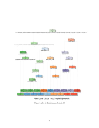
The first task was to determine model fit.
Next, construct a Decision Tree graph
fancyRpartPlot(modelFit)
Next, I used the predict function for model fitting.
3
5. predict_perf<- predict(modelFit, testing, type = "class")
Lastly, I used a confusion matrix to test the results.
confusionMatrix(predict_perf, testing$classe)
## Confusion Matrix and Statistics
##
## Reference
## Prediction A B C D E
## A 2154 62 3 3 0
## B 58 1237 67 60 0
## C 19 206 1271 144 58
## D 0 13 27 1011 166
## E 0 0 0 68 1218
##
## Overall Statistics
##
## Accuracy : 0.8784
## 95% CI : (0.871, 0.8855)
## No Information Rate : 0.2844
## P-Value [Acc > NIR] : < 2.2e-16
##
## Kappa : 0.8463
## Mcnemar's Test P-Value : NA
##
## Statistics by Class:
##
## Class: A Class: B Class: C Class: D Class: E
## Sensitivity 0.9655 0.8149 0.9291 0.7862 0.8447
## Specificity 0.9879 0.9708 0.9341 0.9686 0.9894
## Pos Pred Value 0.9694 0.8699 0.7485 0.8307 0.9471
## Neg Pred Value 0.9863 0.9563 0.9842 0.9585 0.9658
## Prevalence 0.2844 0.1935 0.1744 0.1639 0.1838
## Detection Rate 0.2746 0.1577 0.1620 0.1289 0.1553
## Detection Prevalence 0.2832 0.1813 0.2164 0.1551 0.1639
## Balanced Accuracy 0.9767 0.8928 0.9316 0.8774 0.9170
The output for this approach is not too bad. Overall model accuracy was 0.8711 or 87.11%. Within a 95%
probability, the model accuracy ranges between 0.8635 and 0.8785. This test is confirmed by a p-value < 0.05.
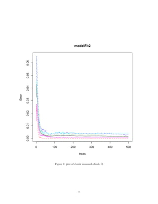
Machine learning using Random Forests
Like the previous analysis, I wanted to determine model fit. This time instead of using the Decision Tree
approach, I used the randomForest function.
modelFit2<- randomForest(classe ~., data = training)
Next, I wanted to predict the in-sample error.
predict_perf2<- predict(modelFit2, testing, type = "class")
And once again, the last step was to use a confusion matrix to test results.
confusionMatrix(predict_perf2, testing$classe)
5
6. ## Confusion Matrix and Statistics
##
## Reference
## Prediction A B C D E
## A 2231 0 0 0 0
## B 0 1518 1 0 0
## C 0 0 1367 3 0
## D 0 0 0 1279 0
## E 0 0 0 4 1442
##
## Overall Statistics
##
## Accuracy : 0.999
## 95% CI : (0.998, 0.9996)
## No Information Rate : 0.2844
## P-Value [Acc > NIR] : < 2.2e-16
##
## Kappa : 0.9987
## Mcnemar's Test P-Value : NA
##
## Statistics by Class:
##
## Class: A Class: B Class: C Class: D Class: E
## Sensitivity 1.0000 1.0000 0.9993 0.9946 1.0000
## Specificity 1.0000 0.9998 0.9995 1.0000 0.9994
## Pos Pred Value 1.0000 0.9993 0.9978 1.0000 0.9972
## Neg Pred Value 1.0000 1.0000 0.9998 0.9989 1.0000
## Prevalence 0.2844 0.1935 0.1744 0.1639 0.1838
## Detection Rate 0.2844 0.1935 0.1743 0.1630 0.1838
## Detection Prevalence 0.2844 0.1936 0.1746 0.1630 0.1843
## Balanced Accuracy 1.0000 0.9999 0.9994 0.9973 0.9997
Model accuracy is 0.9994 or 99.94% with a 95% probability that the model has an accuracy between 0.9985
and 0.9998. This test is confirmed by a p-value of < 0.05.
plot(modelFit2)
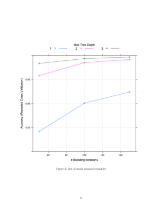
Machine learning using Boosted Regressions
set.seed(2058)
fitControl <- trainControl(method = "repeatedcv",number = 5, repeats = 1)
gbmFit <- train(classe ~ ., data=training, method = "gbm",
trControl = fitControl,
verbose = FALSE)
gbmFinMod <- gbmFit$finalModel
gbmPredTest <- predict(gbmFit, newdata=testing)
gbmAccuracyTest <- confusionMatrix(gbmPredTest, testing$classe)
gbmAccuracyTest
## Confusion Matrix and Statistics
6
8. ##
## Reference
## Prediction A B C D E
## A 2231 1 0 0 0
## B 0 1513 0 0 0
## C 0 3 1354 6 0
## D 0 1 14 1275 1
## E 0 0 0 5 1441
##
## Overall Statistics
##
## Accuracy : 0.996
## 95% CI : (0.9944, 0.9973)
## No Information Rate : 0.2844
## P-Value [Acc > NIR] : < 2.2e-16
##
## Kappa : 0.995
## Mcnemar's Test P-Value : NA
##
## Statistics by Class:
##
## Class: A Class: B Class: C Class: D Class: E
## Sensitivity 1.0000 0.9967 0.9898 0.9914 0.9993
## Specificity 0.9998 1.0000 0.9986 0.9976 0.9992
## Pos Pred Value 0.9996 1.0000 0.9934 0.9876 0.9965
## Neg Pred Value 1.0000 0.9992 0.9978 0.9983 0.9998
## Prevalence 0.2844 0.1935 0.1744 0.1639 0.1838
## Detection Rate 0.2844 0.1929 0.1726 0.1625 0.1837
## Detection Prevalence 0.2845 0.1929 0.1737 0.1646 0.1843
## Balanced Accuracy 0.9999 0.9984 0.9942 0.9945 0.9993
Model accuracy is 0.996 or 99.6% with a 95% probability that model has an accuracy between 0.9944 and
0.9973.
plot(gbmFit, ylim=c(0.80, 1))
After running the Decision Tree, Random Forest and GBM frameworks, I’ve come to the conclusion that
Random Forests is the optimal approach.
Decision Tree error rate: 12.89% Random Forests error rate: 0.06% General Boosted Regressions error rate:
0.40%
Finally, we will use the Random Forest model for prediction
predict_final<- predict(modelFit2, testing, type = "class")
##
##
## processing file: Peterson - Machine Learning Project.Rmd
## Error in parse_block(g[-1], g[1], params.src): duplicate label 'setup'
8