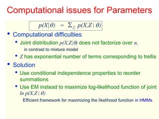
This document discusses hidden Markov models (HMMs) and their parameters. It contains the following key points:
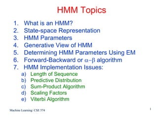
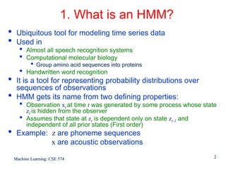
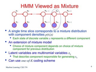
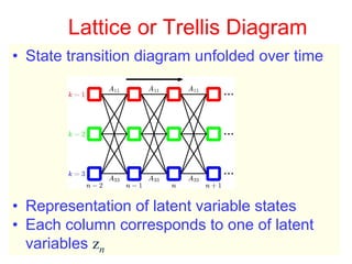
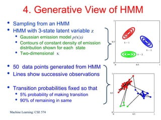
1. HMMs are statistical models used to model time series data. They have hidden states that generate observed outputs.
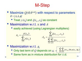
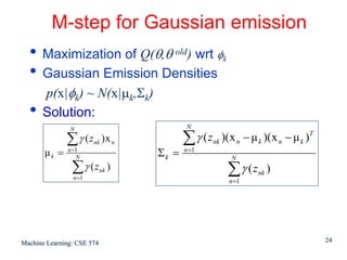
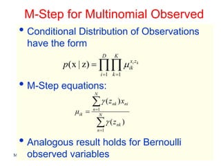
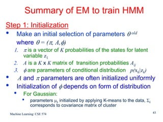
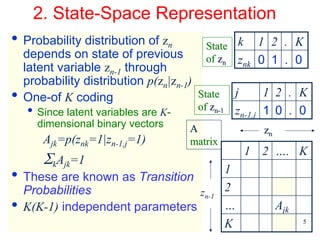
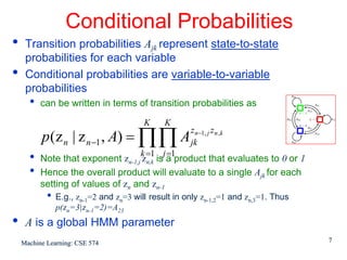
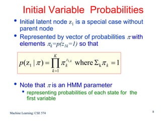
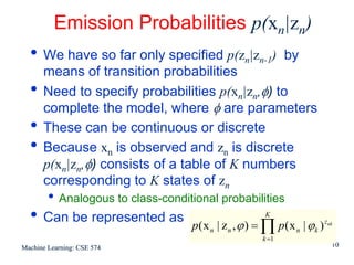
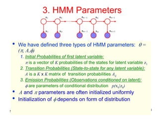
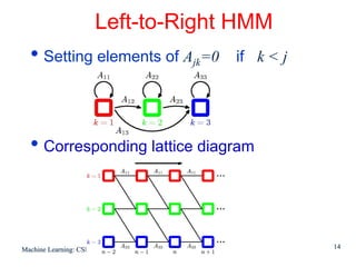
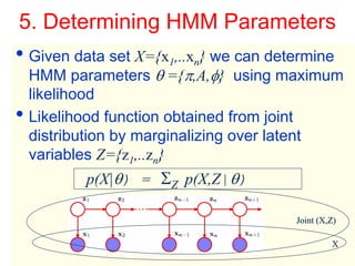
2. HMMs have three main parameters: initial state probabilities, transition probabilities between states, and emission probabilities of observations given states.
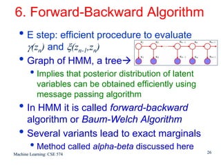
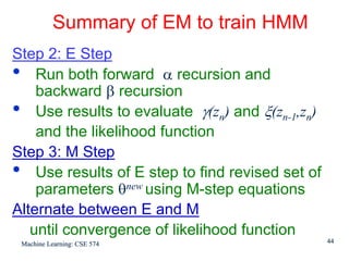
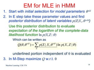
3. The Expectation-Maximization (EM) algorithm is commonly used to estimate HMM parameters from observed data by iteratively computing expected state probabilities.


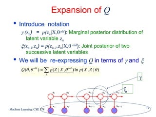
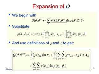
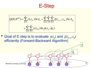
![Detail of γ and ξ
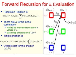
For each value of n we can store
γ(zn) using K non-negative numbers that sum to unity
ξ(zn-1,zn) using a K x K matrix whose elements also sum
to unity
• Using notation
γ (znk) denotes conditional probability of znk=1
Similar notation for ξ(zn-1,j,znk)
• Because the expectation of a binary random
variable is the probability that it takes value 1
γ(znk) = E[znk] = Σz γ(z)znk
ξ(z ,z ) = E[zn-1,j,znk] = Σz γ(z) zn-1,jznk
n-1,j nk
Machine Learning: CSE 574 20](https://image.slidesharecdn.com/powerpoint-presentation2324/85/PowerPoint-Presentation-21-320.jpg)