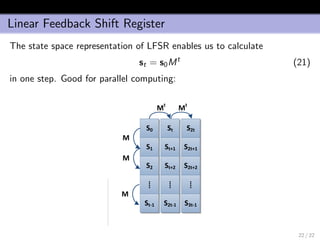
Download to read offline

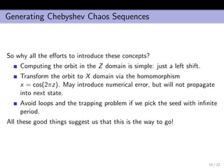
![Chebyshev Dynamic System
Definition
The Chebysheb Dynamic System of degree p is a quadruple
(X, A, ρ(x), Tp) (1)
where
1. X = [−1, 1],
2. A is the Borel σ-algebra on X,
3. ρ(x) = 1
π
√
1−x2
is the density of the invariant measure.
4. Tp : X → X is the Chebyshev polynomial of degree p.
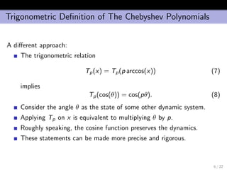
Example:
T2(x) = 2x2
− 1. (2)
2 / 22](https://image.slidesharecdn.com/2012-05-04slidesgeneratingchebychevchaoticsequence-150903203036-lva1-app6891/85/Generating-Chebychev-Chaotic-Sequence-2-320.jpg)
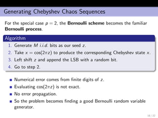
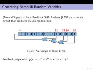

The document discusses generating Chebyshev chaotic sequences through a defined dynamic system, including properties like mixing and ergodicity. It presents challenges like numerical errors due to finite precision in computers and introduces methods for generating irrational seeds and Bernoulli random variables effectively for simulation. Lastly, it highlights the use of linear feedback shift registers (LFSR) as a way to obtain pseudo-random bits for forming the chaotic sequences.