This document discusses the application of graph theory in electric circuit analysis. It explains how to convert an electric circuit into an oriented graph by representing each element as a line segment between nodes. Key graph theory terms are defined such as elements, nodes, branches, trees, and links. Different matrix representations are derived from the oriented graph, including the element node incidence matrix, reduced incidence matrix, basic loop matrix, and basic cut-set matrix. Procedures for using these matrices to solve circuits using Kirchhoff's voltage and current laws are provided.

1. Circuit Theory-I, Lecture Note updated: Autumn Semester 2020 prepared by chekudorji.cst@rub.edu.bt
Application of Graph Theory in Electric Circuit Analysis
Consider an electric circuit shown in figure (01) and it is being converted into oriented graph shown in figure
(02);
1. Graph: It is the geometrical interconnection of the elements of a network.
1R
2R
3R
4R
5R
1e
2e
3e
5e
4e
O
1
2
3
Vs
Figure 01 an actual Circuit
Figure 02 The oriented graph
2. Element (e): it is a component of network, every element is represented by a line segment between two
nodes. Example in figure 01, the resistors and sources are the elements of a graph.
3. Node (n): The end points of the line segments (n)
4. Oriented graph: If each element of the connected graph is assigned a direction, it’s called an oriented
graph or directed graph.
5. Branches: A subset of the elements which make tree and co-trees.
Number of branches required to form a tree is given by b=n-1
Where b is number of branches
n is number of nodes
In figure 02 elements e1, e3 and e5 are the branches.
6. Tree: it is a connected graph containing branches and all the nodes but no closed path
1e
3e
5e
O
1 3
Figure 03 Tree
1e
2e
5e
O
1 3
Figure 04 Co-Tree
7. Co-Trees: Those links which can also form tree by swapping branches and links elements. Figure 04 is
co-tree to figure 03 and vice-versa.

2. Circuit Theory-I, Lecture Note updated: Autumn Semester 2020 prepared by chekudorji.cst@rub.edu.bt
8. Links (l): Those elements of the connected graph that are not included in tree.
Number of links is given, l = e-b
Where e is number of elements
1e
2e
3e
5e
4e
O
1
2
3
Figure 05 branches and links
1L
2L
In figure (05) elements e2, e5 are links and e1, e3, e5 are branches. If a link is added to branches it forms a loop.
Types of Matrices from Graph Theory
The following matrices are derived from the oriented graph;
1. Element node incidence matrix [A]
2. Bus reduced incidence matrix [𝑨̅]
3. Basic loop or Tie-set incidence matrix [B]
4. Basic cut-set incidence matrix [C]
ne 1 2 3 4 5
0 1 1 1
1 -1 1
2 -1 -1 1
3 -1 -1
Note: element directed away from node is positive (+1) and in-coming is negative (-1)
[𝐴]=

3. Circuit Theory-I, Lecture Note updated: Autumn Semester 2020 prepared by chekudorji.cst@rub.edu.bt
ne 1 2 3 4 5
1 -1 1
2 -1 -1 1
3 -1 -1
[A̅] is obtained when first raw of matrix [A] is removed, i.e element crossponding to reference node is removed.
1e
2e
3e
5e
4e
O
1
2
3
Figure 05 branches and links
1L
2L
loope 1 2 3 4 5
L1 1 1 -1
L2 1 1 -1
Note: loop is directed in the direction of link, no. of loops= no. of links.
[𝐴̅]=
[𝐵]=

4. Circuit Theory-I, Lecture Note updated: Autumn Semester 2020 prepared by chekudorji.cst@rub.edu.bt
1e
2e
3e
5e
4e
O
1
2
3
Figure 06 branches and cutsets
1L1C
2C
3C
Cute 1 2 3 4 5
C1 1 -1
C2 1 1 -1
C3 1 1
Note: Cut-set is directed in direction of branch. At least one link should be cut along with branch
Number of cut sets is equal to number of branches.
Procedure to solve electric circuits using Graph Theory
1. Identify the no. of nodes including reference node of the primitive network (a node will connect two or
more elements, each element is represented by a line segment in the graph)
2. Convert network into oriented graph (elements are directed in the actual direction of current flow in the
circuits)
3. Voltage source is short circuited and current source is open circuited ( Current source being O.C. it
will not form element in the graph)
4. . Compute number of branches (b), elements (e) and links (l)
5. . Choose a tree and identify the branches and links
6. Deduce the incidence matrix [A] and Reduced incidence matrix [𝐴̅ ]
7. Deduce tie-set Matrix [B].
8. Deduce cut-set Matrix [C].
Application of Graph Matrices:
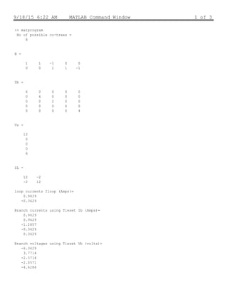
1. Reduced incidence matrix [𝑨̅ ]
The determinant of product of [𝐴̅ ] [𝐴̅ 𝑇
] gives number of possible co-trees
i.e |𝐴̅ 𝐴̅ 𝑇|= No. of Possible co-trees of a graph
[𝐶]=

5. Circuit Theory-I, Lecture Note updated: Autumn Semester 2020 prepared by chekudorji.cst@rub.edu.bt
 The connectivity of the network or the connected graph can be also reconstructed from the matrix
[𝐴̅ ], by adding 1 or 0 to make the sum of each column in the matrix equal to zero.
2. Tie-set Matrix [B] is applicable to KVL to solve mesh circuits and compute
i) loop currents, IL (mx1 matrix size)
ii) Branch currents (ib) and branch Vb) voltage of the circuits
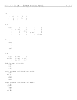
3. Cut-set Matrix [C] is applicable to KCL to solve nodal circuits and compute
(i) Nodal Voltages, Vn (mx1 matrix size)
(ii) branch voltage (Vb) and Branch currents (ib) of the circuits
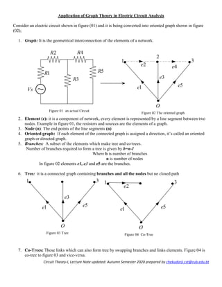
1. Tie-set matrix [B] and KVL equations
Consider a primitive network having many branch elements and sources as shown in figure (i)
1Vs 2Vs
3Vs
1bZ
2bZ
3bZ
5bZ
6bZ
Fig.(i)
bi
bi
bi
bi
bi
bi
bi
bi
bZ
By KVL, the algebraic sum of voltages 𝑉𝑙 in every loop is zero
∑ 𝑉𝑙 = 0
i.e ∑ 𝐵𝑉𝑠 = 0
Where 𝑉𝑠 is voltage across each element, with matrix size (mx1)
The loop equation in terms of loop impedance (𝑍𝑙) and loop current (𝐼𝑙) may be written as
𝑍𝑙 𝐼𝑙 = 𝑉𝑙 (1)
Multiplying equation (1) using tie-set matrix [B]
𝑍𝑙 = 𝐵𝑍 𝑏 𝐵 𝑇
, Where 𝑍 𝑏 𝑖𝑠 𝑡ℎ𝑒 𝑏𝑟𝑎𝑛𝑐ℎ 𝑖𝑚𝑝𝑒𝑑𝑎𝑛𝑐𝑒 𝑜𝑟 𝑠𝑒𝑙𝑓 𝑖𝑚𝑝𝑒𝑑𝑎𝑛𝑐𝑒 𝑜𝑓 𝑒𝑎𝑐ℎ 𝑒𝑙𝑒𝑚𝑒𝑛𝑡
The source voltage 𝑉𝑙 in a loop multiply by tie-set matrix [B]
𝑉𝑙 = 𝐵𝑉𝑠, size (mx1)
(Note: Vs is Positive, if element is oriented in same direction of positive terminal of Vs.

6. Circuit Theory-I, Lecture Note updated: Autumn Semester 2020 prepared by chekudorji.cst@rub.edu.bt
Vs is negative, if element is oriented in opposite direction of positive terminal of Vs)
Therefore equation (1) may be rewritten as
𝐵𝑍 𝑏 𝐵 𝑇
𝐼𝑙 = 𝐵𝑉𝑠 (2) Known as the matrix loop equation
Where [B] of matrix 𝑚𝑥𝑛
𝑍 𝑏 𝑜𝑓 𝑚𝑎𝑡𝑟𝑖𝑥 𝑚𝑥𝑚
𝐼𝑙 𝑜𝑓 𝑚𝑎𝑡𝑟𝑖𝑥 𝑚𝑥1
𝑉𝑠 𝑜𝑓 𝑚𝑎𝑡𝑟𝑖𝑥 𝑚𝑥1
The relation between branch currents(𝑖 𝑏) and loop current (𝐼𝑙) may be derived as
𝑖 𝑏 = 𝐵 𝑇
𝐼𝑙 (3)
And branch voltages derived as
𝑉𝑏 = 𝑍 𝑏 𝑖 𝑏 − 𝑉𝑠 (4)
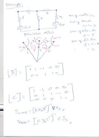
2. Cut-Set Matrix [C] and KCL equations
Consider a primitive admittance network having many node elements and current sources as shown in fig.(ii)
2Is
3Is
2bY
3bY
5bY
6bY
Fig.(ii)
1Is
bi
bi
bi
bi
bi
bi
1Vn 2Vn 3Vn
By KCL, the algebraic sum of branch currents in every node is zero
∑ 𝐼 𝑛 = 0
i.e ∑ 𝐶𝐼𝑠 = 0
Where 𝐼𝑠 is current source flowing in each element, with matrix size (mx1)
The nodal equation in terms of admittance (𝑌𝑛) and nodal voltage (𝑉𝑛) may be written as
𝑌𝑛 𝑉𝑛 = 𝐼 𝑛 (1)
Multiplying equation (1) using cut-set matrix [C]
𝑌𝑛 = 𝐶𝑌𝑏 𝐶 𝑇
, Where 𝑌𝑏 𝑖𝑠 𝑡ℎ𝑒 𝑏𝑟𝑎𝑛𝑐ℎ 𝑎𝑑𝑚𝑖𝑡𝑡𝑎𝑛𝑐𝑒 𝑜𝑟 𝑠𝑒𝑙𝑓 𝑎𝑑𝑚𝑖𝑡𝑡𝑎𝑛𝑐𝑒 𝑜𝑓 𝑒𝑎𝑐ℎ 𝑒𝑙𝑒𝑚𝑒𝑛𝑡

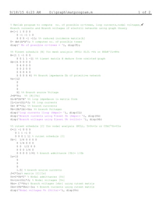
7. Circuit Theory-I, Lecture Note updated: Autumn Semester 2020 prepared by chekudorji.cst@rub.edu.bt
The source current multiply by cut-set matrix [C]
𝐼 𝑛 = 𝐶𝐼𝑠
Therefore equation (1) may be rewritten as
𝐶𝑌𝑏 𝐶 𝑇
𝑉𝑛 = 𝐶𝐼𝑠 (2) Known as the matrix nodal equation
Where [C] of matrix 𝑚𝑥𝑛
𝑌𝑏 𝑜𝑓 𝑚𝑎𝑡𝑟𝑖𝑥 𝑚𝑥𝑚
𝐼 𝑛 𝑜𝑓 𝑚𝑎𝑡𝑟𝑖𝑥 𝑚𝑥1
𝑉𝑛 𝑜𝑓 𝑚𝑎𝑡𝑟𝑖𝑥 𝑚𝑥1
The relation between branch voltages (𝑣 𝑏) and nodal voltages (𝑉𝑛) may be derived as
𝑣 𝑏 = 𝐶 𝑇
𝑉𝑛 (3)
And branch currents as
𝑖 𝑏 = 𝑌𝑏 𝑣 𝑏 − 𝐼𝑠 (4)

8. -