This document summarizes a group project on impedance matching and tuning. It discusses using transformers on transmission lines to match the signal impedance to the load impedance. It describes several methods for impedance matching - using a quarter wave transformer, L-network matching, discrete elements, single stub tuning, and double stub tuning. It provides examples of applying these different matching techniques and shows the resulting simulation plots and solutions. It also discusses the group's process for completing the project, including researching the techniques, developing the MATLAB code, and testing the results.

1. 1
ELECTRICAL ENGINEERING
VCU School of Engineering
EGRE 310 – Microwave and Photonics Engineering
Group Project, Spring 2015
Impedance Matching and Tuning
Group Members
Jacob M. Ramey
Ngoc Hue Vo
Honor Pledge:We have neither given nor received any unauthorized help on this project.
Signed:
____________________ ____________________

2. 2
I. Introduction
The purpose of this project was to study the use of transformers on a transmission line that can be
used to ‘match’ a signal to a line. Signal matching is done to maximize the amount of power delivered
to the load by varying the impedance at the input of the load.
II. Background & Theory:
Impedance matching and tuning can be done in many ways – In this project we utilize at least
4 types. The different types of matching are used depending on the project guidelines and limitations.
A quarter wave transformer, an L network, discrete element matching, single stub tuning, and double
stub tuning are all possible ways to approach this problem.
The first one, perhaps the simplest to understand and implement (though not always feasible)
– the quarter wave transformer. We use smith chart operations to determine the length away from the
load the transformer needs to be placed and then calculate the required characteristic impedance of
the transformer using the equation 𝑍 𝜆
4
= √ 𝑍 𝐿 𝑍0 where Z0 is the characteristic impedance of the line.
L- Network matching is done by using purely reactive elements to bring the reflection
coefficient of the load to zero (or ‘close enough’). The goal is of course to have zero reflection. The
importance of the Smith chart once again comes in to place when working with this approach.
Depending on the location of the normalized load impedance on the chart, there will be 2 or 4
solutions. The R=1 circle and the mirror image G=1 circle are the boundaries for determining the
solutions and the number of them that will occur. If the load impedance is inside either the R=1 or
G=1 circle, then there will be 2 solutions. If the elsewhere (outside the circles) then there will be 4
solutions. The solutions are found be starting at the load impedance and traveling along the reactance
lines until they reach R=1 or G=1. At this point the solution is changed to the reciprocal (admittance
to impedance or vice versa) and another reactive element is added (this way is stays on the R=1 circle)
and the reactivity of the line is effectively matched with the complex conjugate of the lines imaginary
impedance or admittance.
The matching of a transmission line with the load can be done using discrete components or
elements called stubs which are small pieces of transmission lines that are either shorts or open
circuits with lengths comparable to the wavelength of the frequency of operation. The discrete
components are just the commonly capacitors, inductors, and other lumped elements we use every
day. Stubs are use commonly at high frequencies because the size of the stubs is small enough to be
effective and also to reduce costs.
Sometimes when working with a single stub we are faced with a huge limitation – we cannot
easily change or tune our stubs to fit any other frequencies. This is where double stubs and multi stub
networks come into play. A double stub network places two stubs at an arbitrary distance away from
the load at a distance ‘d’ apart from each other. The first stub is used to bring the transmission lines
input impedance to a solution on the Smith chart corresponding the G=1 or R=1 circle, the space ‘d’
must be account for between the stubs, then the second stub is used to bring the input impedance to a
purely real and matched state where the reflection coefficient is zero. This will maximize our power.
Program Specifications:
- Z0 , the characteristic impedance of the line.
- ZL, the line impedance
- 𝑓 , the frequency of operation.

3. 3
III. Simulation Results:
Below are two examples with different loads. One plot and two console outputs are provided
due to considerations regarding limited space allotted for the report. On the Smith Charts, a green dot
indicates the complex reflection coefficient at the start frequency while the red dot indicates the value
at the stop frequency. The first example demonstrates where the impedance is inside the r=1 circle.
The second example was chosen to compare directly with a sample provided in the Ulaby textbook.
Quarter Wavelength Transformer (2)
Solution 1:
d1 = 0.1349 lambda = 404.6876 mm
Z(d1) = 11.721778 Ohms
Z(lambda/4) = 24.209273 Ohms
Solution 2:
d2 = 0.3849 lambda = 1154.6876 mm
Z(d2) = 213.278222 Ohms
Z(lambda/4) = 103.266215 Ohms
Transformer Length = 750.000000 mm
L - Network Matching Solutions (2)
Case 2: Inside r=1 circle
Solution 1:
X1 = 75.0000 Ohms
L1 = 119.366207 nH
B1 = 0.0200 Siemens
C2 = 31.830989 pF
Bandwidth: 26.10 MHz
Solution 2:
X2 = 25.0000 Ohms
L1 = 39.788736 nH
B2 = -0.0200 Siemens
L2 = 79.577472 nH
Bandwidth: 29.12 MHz

4. 4
Single Stub Solutions (4):
Solution 1:
0.030711 m shunt short-circuit stub at 0.064012 m from the load
Bandwidth: 149.74 MHz
Solution 2:
0.11929 m shunt short-circuit stub at 0.11092 m from the load
Bandwidth: 65.13 MHz
Solution 3:
0.044289 m shunt open-circuit stub at 0.11092 m from theload
Bandwidth: 89.95 MHz
Solution 4:
0.10571 m shunt open-circuit stub at 0.064012 m from theload
Bandwidth: 788.96 MHz
Discrete Element Solutions (2):
Solution 1:
5.9646e-09 H shunt inductor at 0.064012 m from the load
Bandwidth: 158.86 MHz
Solution 2:
4.2468e-12 F shunt capacitor at 0.11092 m from the load
Bandwidth: 98.79 MHz

5. 5
IV. Discussion:
The examples we’ve chosen to show were selected specifically because we had known
solutions for the parameters on hand. We used these known solutions, as well as the amanogowa
website to confirm our results for each of the solution types. While we know that the solutions
outputted to the console are correct, the plots themselves require interpretation to confirm that they
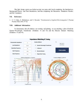
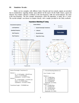
are too correct. One thing we noticed is that the Smith Chart plot repeated crosses over the real axis,
and the number of times it crosses is equal to the number of peaks on the reflection magnitude vs.
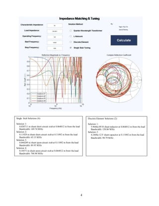
frequency plot, which is one way to check that the plots makes sense. The plots for single stub and
quarter-wavelength transformer were interesting because they have frequency dependence, and so in
the magnitude of reflection vs. frequency plot, they both have numerous peaks, whereas the element
dependent solutions have a single peak.
V. Conclusions:
By deriving and programming analytical solutions for impedance matching problems, we’ve
gained a greater familiarity with the process for all four of the solution types. Most significantly,
we’ve learned a lot of MATLAB while working on this project. This application had so many parts
to it and required learning about advanced solution plotting, developing GUIs, and countless other
things that we’ve never experienced in previous courses. Throughout the course of the development
process, it became clear that we needed to focus on modular programming that would enable us both
to easily read and work on the main program (1636 lines of code), which is an important lesson to
learn when performing software development in a team setting. That, along with the experience in
MATLAB were perhaps the most useful and important take-aways from the project.
VI. Task Breakdown & Design Process:
The project was given and we decided that we should break the work up into parts so we could
both tackle it in an efficient manner while still allowing us to complete other. At first, we needed to
do research on the different types of matching so we could figure out exactly what code needed to be
written. The different types of networks that outlined above were assigned to each of us – [Jacob]
worked on quarter wave transformer and L network match while [Hue] worked on the discrete
element matching and stub tuning. After researching for a while we discovered that the majority of
the matching networks were solved in a similar fashion and that researching the topics together proved
more effective. We researched a few sources online and used two books from the class (Pozar, Ulaby)
when figuring out how to design the networks theoretically and mathematically.
The MATLAB implementation took the longest and by far was the most difficult – but with
hard work came results and we were able to get some of the graphs working and all the functions.
The math wasn’t a difficult part of the MATLAB coding or algorithms, but the graphing and GUI
were pretty difficult. The numbers for all the solutions printed out fine in the command window. The
GUI had been made on a desktop computer that had dimensions that were much larger than the laptop
computer which we had presented the material on and this resulted in a problem in the display on the
GUI. After some modifications to the resolution we were able to see the whole window and input the
arguments we need for the problem. The type of solution is to be selected (L network, quarter wave,
etc) and the input arguments specified earlier are to be specified. Pressing the ‘calculate’ button would
generate the results of the solutions numerically in the command window and also print out the
respective graphs in the window. The MATAB coding in its entirety was written together and we
didn’t designate one part of the code for each person but wrote snippets of code and pieced them all
together in the end.

6. 6
This final design report was broken up into two parts with Jacob completing the Introduction,
Background/Theory, and Task Breakdown, and Hue completing the Discussion, Simulation Results,
and the Conclusion.
VII. Reference:
1. F. T. Ulaby, E. Michielssen, and U. Ravaioli, “Fundamentals of Applied Electromagnetics”, Pearson
Prentice Hall, 2010, 6th
Ed.
VIII. Additional Information:
To demonstrate that all solutions are working and plotting, we are attaching a plot of both the
Quarter-Wavelength Transformer (Solutions #1 and #2) and the Discrete Element Matching
(Solutions #3 and #4).