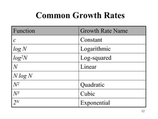
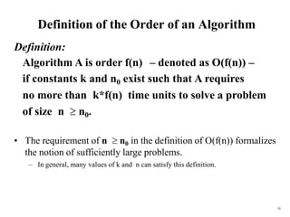
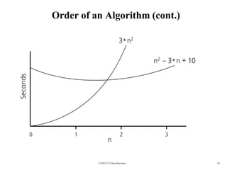
The document discusses algorithm analysis and determining the efficiency of algorithms. It introduces key concepts such as: - Algorithms must be correct and efficient to solve problems. - The time and space complexity of algorithms is analyzed to compare efficiencies. Common growth rates include constant, logarithmic, linear, quadratic, and exponential time. - The asymptotic worst-case time complexity of an algorithm (its "order") is expressed using Big O notation, such as O(n) for linear time. Higher order terms indicate slower growth.

1. Algorithm Analysis
1

2. Algorithm
2
• An algorithm is a set of instructions to be followed to
solve a problem.
– There can be more than one solution (more than one
algorithm) to solve a given problem.
– An algorithm can be implemented using different
programming languages on different platforms.
• An algorithm must be correct. It should correctly solve
the problem.
– e.g. For sorting, this means even if (1) the input is already
sorted, or (2) it contains repeated elements.
• Once we have a correct algorithm for a problem, we
have to determine the efficiency of that algorithm.

3. 3
Algorithmic Performance
There are two aspects of algorithmic performance:
• Time
• Instructions take time.
• How fast does the algorithm perform?
• What affects its runtime?
• Space
• Data structures take space
• What kind of data structures can be used?
• How does choice of data structure affect the runtime?
 We will focus on time:
– How to estimate the time required for an algorithm
– How to reduce the time required

4. 4
Analysis of Algorithms
• Analysis of Algorithms is the area of computer science that
provides tools to analyze the efficiency of different methods of
solutions.
• How do we compare the time efficiency of two algorithms that
solve the same problem?
Naïve Approach: implement these algorithms in a programming
language (C++), and run them to compare their time
requirements. Comparing the programs (instead of algorithms)
has difficulties.

5. 5
Analysis of Algorithms
• When we analyze algorithms, we should employ
mathematical techniques that analyze algorithms
independently of specific
implementations, computers, or data.
• To analyze algorithms:
– First, we start to count the number of significant
operations in a particular solution to assess its
efficiency.
– Then, we will express the efficiency of algorithms
using growth functions.

6. 6
The Execution Time of Algorithms
• Each operation in an algorithm (or a program) has a cost.
 Each operation takes a certain of time.
count = count + 1;  take a certain amount of time, but it is constant
A sequence of operations:
count = count + 1; Cost: c1
sum = sum + count; Cost: c2
 Total Cost = c1 + c2

7. 7
The Execution Time of Algorithms (cont.)
Example: Simple If-Statement
Cost
c1
c2
Times
1
1
if (n < 0)
absval = -n
else
absval = n; c3 1
Total Cost <= c1 + max(c2,c3)

8. 8
The Execution Time of Algorithms (cont.)
Example: Simple Loop
Cost Times
i = 1; c1 1
sum = 0;
while (i <= n) {
c2
c3
1
n+1
i = i
sum =
+ 1;
sum + i;
c4
c5
n
n
}
Total Cost = c1 + c2 + (n+1)*c3 + n*c4 + n*c5
 The time required for this algorithm is proportional to n

9. 9
The Execution Time of Algorithms (cont.)
Example: Nested Loop
Cost Times
i=1; c1 1
sum = 0; c2 1
while (i <= n) { c3 n+1
j=1; c4 n
while (j <= n) { c5 n*(n+1)
sum = sum + i; c6 n*n
j = j + 1; c7 n*n
}
i = i +1; c8 n
}
Total Cost = c1 + c2 + (n+1)*c3 + n*c4 + n*(n+1)*c5+n*n*c6+n*n*c7+n*c8
 The time required for this algorithm is proportional to n2

10. 10
Algorithm Growth Rates
• We measure an algorithm’s time requirement as a function of the
problem size.
– Problem size depends on the application: e.g. number of elements in a list for a
sorting algorithm, the number disks for towers of hanoi.
• So, for instance, we say that (if the problem size is n)
– Algorithm A requires 5*n2 time units to solve a problem of size n.
– Algorithm B requires 7*n time units to solve a problem of size n.
• The most important thing to learn is how quickly the algorithm’s
time requirement grows as a function of the problem size.
– Algorithm A requires time proportional to n2.
– Algorithm B requires time proportional to n.
• An algorithm’s proportional time requirement is known as
growth rate.
• We can compare the efficiency of two algorithms by comparing
their growth rates.

11. Algorithm Growth Rates (cont.)
Time requirements as a function
of the problem size n
11

12. 12
Common Growth Rates
Function Growth Rate Name
c Constant
log N Logarithmic
log2N Log-squared
N Linear
N log N
N2 Quadratic
N3 Cubic
2N Exponential

13. Figure 6.1
Running times for small inputs
13

14. Figure 6.2
Running times for moderate inputs
14

15. 15
Order-of-Magnitude Analysis and Big O
Notation
• If Algorithm A requires time proportional to f(n), Algorithm A is
said to be order f(n), and it is denoted as O(f(n)).
• The function f(n) is called the algorithm’s growth-rate
function.
• Since the capital O is used in the notation, this notation is called
the Big O notation.
• If Algorithm A requires time proportional to n2, it is O(n2).
• If Algorithm A requires time proportional to n, it is O(n).

16. 16
Definition of the Order of an Algorithm
Definition:
Algorithm A is order f(n) – denoted as O(f(n)) –
if constants k and n0 exist such that A requires
no more than k*f(n) time units to solve a problem
of size n  n0.
• The requirement of n  n0 in the definition of O(f(n)) formalizes
the notion of sufficiently large problems.
– In general, many values of k and n can satisfy this definition.

17. 17
Order of an Algorithm
• If an algorithm requires n2–3*n+10 seconds to solve a problem
size n. If constants k and n0 exist such that
k*n2 > n2–3*n+10 for all n  n0 .
the algorithm is order n2 (In fact, k is 3 and n0 is 2)
3*n2 > n2–3*n+10 for all n  2 .
Thus, the algorithm requires no more than k*n2 time units for n 
n0 ,
So it is O(n2)

18. Order of an Algorithm (cont.)
CENG 213 Data Structures 18

19. A Comparison of Growth-Rate Functions
19

20. A Comparison of Growth-Rate Functions (cont.)
20

21. 21
Growth-Rate Functions
O(1)
O(log2n)
Time requirement is constant, and it is independent of the problem’s size.
Time requirement for a logarithmic algorithm increases increases slowly
as the problem size increases.
Time requirement for a linear algorithm increases directly with the size
of the problem.
O(n)
O(n*log2n) Time requirement for a n*log2n algorithm increases more rapidly than
a linear algorithm.
O(n2) Time requirement for a quadratic algorithm increases rapidly with the
size of the problem.
Time requirement for a cubic algorithm increases more rapidly with the
size of the problem than the time requirement for a quadratic algorithm.
As the size of the problem increases, the time requirement for an
exponential algorithm increases too rapidly to be practical.
O(n3)
O(2n)

22. 22
Growth-Rate Functions
• If an algorithm takes 1 second to run with the problem size
8, what is the time requirement (approximately) for that algorithm
with the problem size 16?
• If its order is:
O(1)  T(n) = 1 second
O(log2n)  T(n) = (1*log216) / log28 = 4/3 seconds
O(n)  T(n) = (1*16) / 8 = 2 seconds
O(n*log2n)  T(n) = (1*16*log216) / 8*log28 = 8/3 seconds
O(n2)  T(n) = (1*162) / 82 = 4 seconds
O(n3)  T(n) = (1*163) / 83 = 8 seconds
O(2n)  T(n) = (1*216) / 28 = 28 seconds = 256 seconds

23. CENG 213 Data Structures 23
Properties of Growth-Rate Functions
1. We can ignore low-order terms in an algorithm’s growth-rate
function.
– If an algorithm is O(n3+4n2+3n), it is also O(n3).
– We only use the higher-order term as algorithm’s growth-rate function.
2. We can ignore a multiplicative constant in the higher-order term
of an algorithm’s growth-rate function.
– If an algorithm is O(5n3), it is also O(n3).
3. O(f(n)) + O(g(n)) = O(f(n)+g(n))
– We can combine growth-rate functions.
– If an algorithm is O(n3) + O(4n), it is also O(n3 +4n2)  So, it is O(n3).
– Similar rules hold for multiplication.

24. 24
Growth-Rate Functions – Example1
Cost Times
i = 1; c1 1
sum = 0; c2 1
while (i
i = i
sum =
<= n)
+ 1;
sum +
{
i;
c3
c4
c5
n+1
n
n
}
T(n) = c1 + c2 + (n+1)*c3 + n*c4 + n*c5
= (c3+c4+c5)*n + (c1+c2+c3)
= a*n + b
 So, the growth-rate function for this algorithm is O(n)

25. 25
Growth-Rate Functions – Example2
Cost Times
i=1; c1 1
sum = 0;
while (i <= n) {
j=1;
while (j <= n) {
c2
c3
c4
c5
1
n+1
n
n*(n+1)
sum = sum +
j = j + 1;
}
i = i +1;
i; c6
c7
c8
n*n
n*n
n
}
T(n) = c1 + c2 + (n+1)*c3 + n*c4 + n*(n+1)*c5+n*n*c6+n*n*c7+n*c8
= (c5+c6+c7)*n2 + (c3+c4+c5+c8)*n + (c1+c2+c3)
= a*n2 + b*n + c
 So, the growth-rate function for this algorithm is O(n2)

26. 26
Growth-Rate Functions – Example3
Cost
c1
Times
n+1
n
 ( j  1)
j 1
for (i=1; i<=n; i++)
for (j=1; j<=i; j++) c2
for (k=1; k<=j; k++) c3
x=x+1; c4
T(n)
n
= c1*(n+1) + c2*(  ( j  1)
j 1
n j
) + c3* (   (k  1)
j 1 k 1
) + c4*( )
= a*n3 + b*n2 + c*n + d
 So, the growth-rate function for this algorithm is O(n3)
n j
  (k  1)
j 1 k 1
n j
  k
j 1 k 1
n j
  k
j 1 k 1

27. CENG 213 Data Structures 27
How much better is O(log2n)?
n O(log2n)
16 4
64 6
256 8
1024 (1KB) 10
16,384 14
131,072 17
262,144 18
524,288 19
1,048,576 (1MB) 20
1,073,741,824 (1GB) 30