Downloaded 11 times


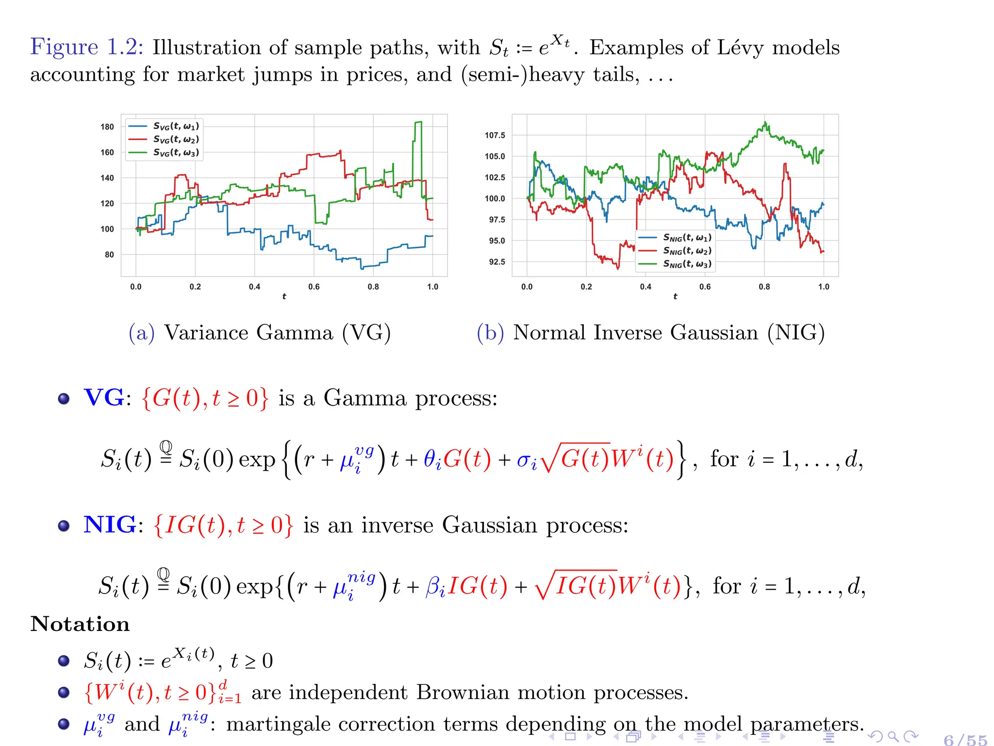
![Framework and Problem Setting
Task: Compute efficiently (up to a discount factor)
E[P(X(T)) ∣ X(0) = x0] = ∫
Rd
P(x) ρXT ∣x0
(x) dx
▸ P ∶ Rd
→ R: payoff function
▸ {Xt ∈ Rd
∶ t ≥ 0}: stochastic processes representing the log-prices of
the underlying assets (resp. risk factors) at time t, defined on a
continuous-time probability space (Ω,F,Q), with Q is the
risk-neutral measure.
Applications in Mathematical Finance: Computing the value
of derivatives (resp. risk measures) depending on multiple assets
(resp. risk factors) and their sensitivities (Greeks).
Features of the problem
P(⋅) is non-smooth.
The dimension d is large.
The pdf, ρXT
, is not known explicitly or expensive to
sample from.
3/55](https://image.slidesharecdn.com/22slidesbenhamouda-250123205348-1bb4dd63/75/Empowering-Fourier-based-Pricing-Methods-for-Efficient-Valuation-of-High-Dimensional-Derivatives-5-2048.jpg)
![Task ((Multi-Asset) Option Pricing and Beyond): Compute efficiently (up to a
discount factor)
E[P(X(T)) ∣ X(0) = x0] = ∫
Rd
P(x) ρXT ∣x0
(x) dx
Setting: Payoff Function
P(⋅): payoff function (typically non-smooth), e.g., (K: the strike price)
▸ Basket put: P(x) = max(K − ∑
d
i=1 ciexi
,0), s.t. ci > 0,∑
d
i=1 ci = 1;
▸ Rainbow (E.g., Call on min): P(x) = max(min(ex1
,...,exd
) − K,0)
▸ Cash-or-nothing (CON) put : P(x) = ∏
d
i=1 1[0,Ki](exi
).
x1
4
2
0
2
4
x
2
4
2
0
2
4
P(x
1
,
x
2
)
0.0
0.2
0.4
0.6
0.8
(a) Basket put
x1
0.0
0.2
0.4
0.6
0.8
1.0
x
2
0.0
0.2
0.4
0.6
0.8
1.0
P
(
x
1
,
x
2
)
0.0
0.2
0.4
0.6
0.8
1.0
1.2
1.4
1.6
(b) Call on min
x1
0
1
2
3
4
5
6
7
x
2
0
1
2
3
4
5
6
7
P(x
1
,
x
2
)
0.0
0.2
0.4
0.6
0.8
1.0
(c) Cash-or-nothing
Figure 1.1: Payoff functions illustration](https://image.slidesharecdn.com/22slidesbenhamouda-250123205348-1bb4dd63/75/Empowering-Fourier-based-Pricing-Methods-for-Efficient-Valuation-of-High-Dimensional-Derivatives-6-2048.jpg)
![Task ((Multi-Asset) Option Pricing and Beyond): Compute efficiently (up to
a discount factor)
E[P(X(T)) ∣ X(0) = x0] = ∫
Rd
P(x) ρXT ∣x0
(x) dx
Setting: Asset Price Model
XT is a d-dimensional (d ≥ 1) vector of log-asset prices at time T,
following a multivariate stochastic model:
▸ Characteristic function, ΦXT
(⋅) ∶= EρXT
[ei⟨⋅,XT ⟩
],
can be known (semi-)analytically or approximated numerically,
e.g,.
☀ Lévy models (Cont et al. 2003): Characteristic function obtained
via Lévy–Khintchine representation.
☀ Affine processes (Duffie et al. 2003): Characteristic function
obtained via Ricatti Equations.
▸ The pdf, ρXT
, is
☀ not known explicitly (e.g. α-stable Lévy processes
(0 < α ≤ 2, α ≠ {1, 1
2
, 2}) (Eberlein 2009)), or
☀ expensive to sample from (e.g. non-Markovian models such
as rough Heston (El Euch et al. 2019)).
5/55](https://image.slidesharecdn.com/22slidesbenhamouda-250123205348-1bb4dd63/75/Empowering-Fourier-based-Pricing-Methods-for-Efficient-Valuation-of-High-Dimensional-Derivatives-7-2048.jpg)
![Numerical Integration Methods
Task ((Multi-Asset) Option Pricing and Beyond): Compute
efficiently (up to discount factor)
E[P(X(T)) ∣ X(0) = x0] = ∫
Rd
P(x) ρXT ∣x0
(x) dx
Features of the problem
P(⋅) is non-smooth.
The dimension d is large.
The pdf, ρXT
, is not known explicitly or expensive to
sample from.
Challenges
1 Monte Carlo method has a convergence rate independent of the
problem’s dimension and integrand’s regularity BUT can be very slow.
2 non-smoothness of P(⋅) and the high dimensionality ⇒ deteriorated
convergence of deterministic quadrature methods.](https://image.slidesharecdn.com/22slidesbenhamouda-250123205348-1bb4dd63/75/Empowering-Fourier-based-Pricing-Methods-for-Efficient-Valuation-of-High-Dimensional-Derivatives-9-2048.jpg)
![Numerical Integration Methods: Sampling in [0,1]2
E[P(X(T))] = ∫Rd P(x)ρXT
(x)dx ≈ ∑
M
m=1 ωmP (Ψ(um)) (Ψ ∶ [0,1]d
→ Rd
).
Monte Carlo (MC)
0 0.2 0.4 0.6 0.8 1
u1
0
0.1
0.2
0.3
0.4
0.5
0.6
0.7
0.8
0.9
1
u2
Tensor Product Quadrature
0 0.2 0.4 0.6 0.8 1
u1
0
0.1
0.2
0.3
0.4
0.5
0.6
0.7
0.8
0.9
1
u2
Quasi-Monte Carlo (QMC)
0 0.2 0.4 0.6 0.8 1
u1
0
0.1
0.2
0.3
0.4
0.5
0.6
0.7
0.8
0.9
1
u2
Adaptive Sparse Grids Quadrature
0 0.2 0.4 0.6 0.8 1
u1
0
0.1
0.2
0.3
0.4
0.5
0.6
0.7
0.8
0.9
1
u2](https://image.slidesharecdn.com/22slidesbenhamouda-250123205348-1bb4dd63/75/Empowering-Fourier-based-Pricing-Methods-for-Efficient-Valuation-of-High-Dimensional-Derivatives-10-2048.jpg)
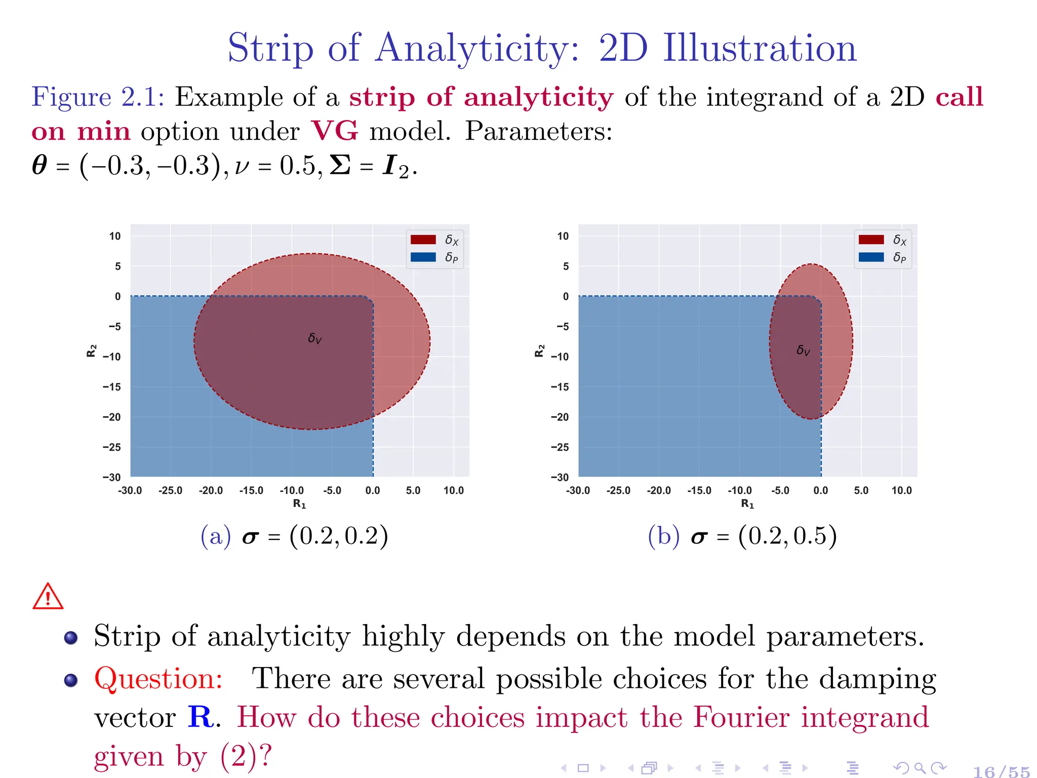
![Fourier Pricing Formula in d Dimensions
Assumption 2.1
1 x ↦ P(x) is continuous on Rd
(can be replaced by additional assumptions on XT ).
2 δP ∶= {R ∈ Rd
∶ x ↦ eR′x
P(x) ∈ L1
bc(Rd
) and y ↦ ̂
P(y + iR) ∈ L1
(Rd
)} ≠ ∅.
(strip of analyticity of ̂
P(⋅))
3 δX ∶= {R ∈ Rd
∶ y ↦∣ ΦXT
(y + iR) ∣< ∞,∀ y ∈ Rd
} ≠ ∅. (strip of analyticity of ΦXT (⋅))
Proposition (Ben Hammouda et al. 2023 (Extension of (Lewis 2001) in 1D and based on
(Eberlein et al. 2010))
Under Assumptions 1, 2 and 3, and for R ∈ δV ∶= δP ∩ δX, the option value on d stocks is
V (ΘX,Θp) ∶= e−rT
E[P(XT)] = ∫
Rd
P(x) ρXT
(x) dx (1)
= (2π)−d
e−rT
∫
Rd
R(ΦXT
(y + iR) ̂
P(y + iR))dy.
Notation
ΘX,Θp: the model and payoff parameters, respectively;
̂
P(⋅): the extended Fourier transform of the payoff P(⋅) ( ̂
P(z) ∶= ∫Rd e−iz′
⋅x
P(x)dx, for z ∈ Cd
);
XT : vector of log-asset prices at time T, with extended characteristic function ΦXT
(⋅) (i.e.,
Φ ∶= ̂
ρ);
R ∈ Rd
: damping parameters ensuring integrability and controlling the integration contour.
R[⋅]: real part of the argument. i: imaginary unit. 12/55](https://image.slidesharecdn.com/22slidesbenhamouda-250123205348-1bb4dd63/75/Empowering-Fourier-based-Pricing-Methods-for-Efficient-Valuation-of-High-Dimensional-Derivatives-15-2048.jpg)
![Fourier Pricing Formula in d Dimensions
Proof (Ben Hammouda et al. 2023).
Using the inverse generalized Fourier transform and Fubini theorems:
V (ΘX,ΘP ) = e−rT
E[P(XT)]
= e−rT
E[(2π)−d
R(∫
Rd
ei(y+iR)′
XT ̂
P(y + iR)dy)], R ∈ δP
= (2π)−d
e−rT
R(∫
Rd
E[ei(y+iR)′
XT
] ̂
P(y + iR)dy), R ∈ δV ∶= δP ∩ δX
= (2π)−d
e−rT
∫
Rd
R(ΦXT
(y + iR) ̂
P(y + iR))dy, R ∈ δV
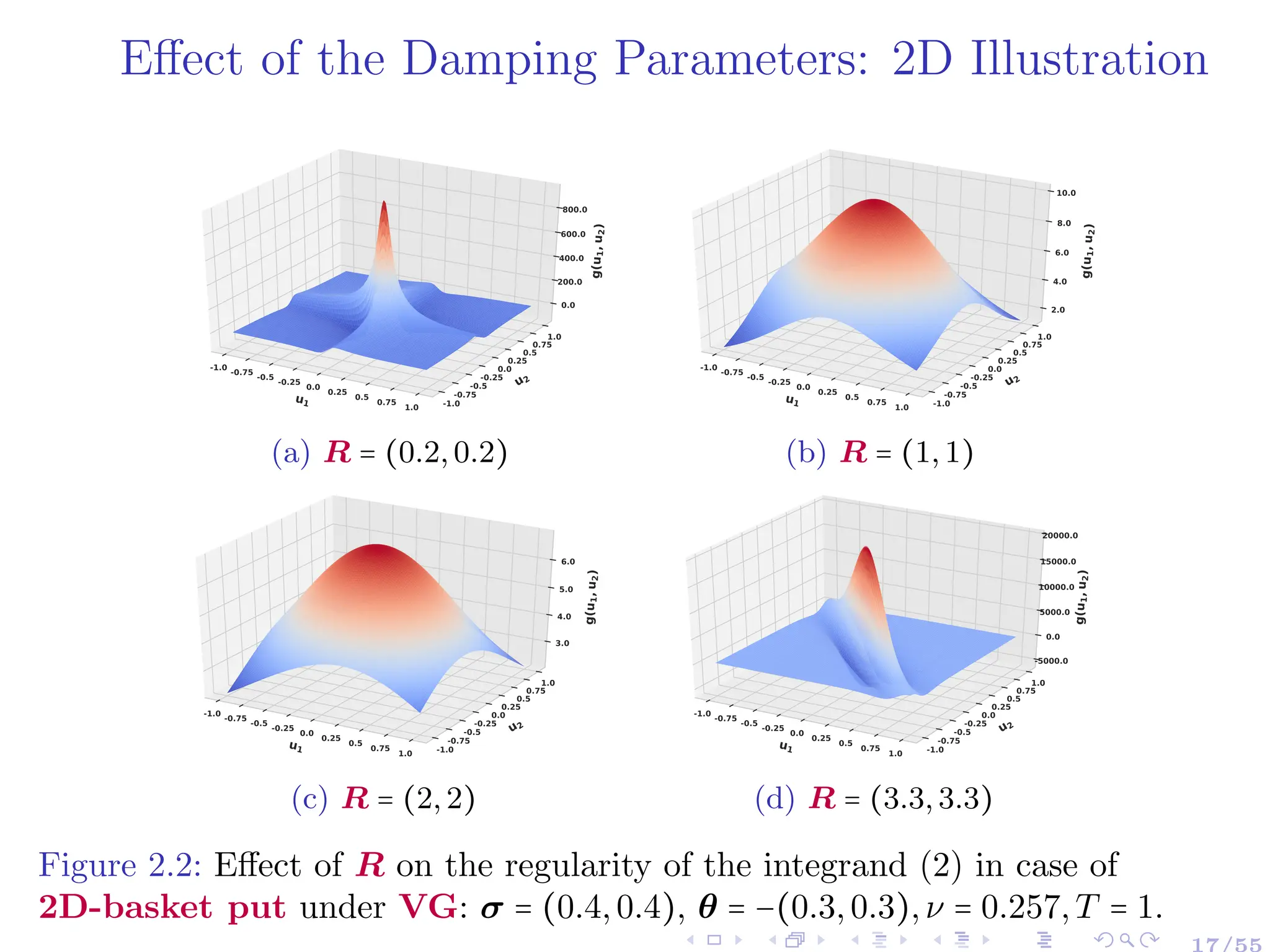
Notation 2.2 (Integrand)
Given R ∈ δV ⊆ Rd
, we define the integrand of interest by
g (y;R,ΘX,ΘP ) ∶= (2π)−d
e−rT
R[ΦXT
(y + iR) ̂
P(y + iR)], y ∈ Rd
, (2)
13/55](https://image.slidesharecdn.com/22slidesbenhamouda-250123205348-1bb4dd63/75/Empowering-Fourier-based-Pricing-Methods-for-Efficient-Valuation-of-High-Dimensional-Derivatives-16-2048.jpg)
![Characteristic Functions: Illustrations
Table 1: ΦXT
(z) = exp(iz′
(X0 + (r + µ)T))ϕXT
(z): extended characteristic function of various
pricing models. I[⋅]: the imaginary part of the argument. Kλ(⋅) is the Bessel function of the
second kind. GH coincides with NIG for λ = −1
2
.
Model ϕXT
(z),z ∈ Cd
, I[z] ∈ δX
GBM exp(−T
2
z′
Σz)
VG (1 − iνz′
θ + 1
2
νz′
Σz)
−T /ν
GH ( α2
−β⊺
∆β
α2−β⊺
∆β+z⊺∆z−2iβ⊺
∆z
)
λ/2 Kλ(δT
√
α2−β⊺
∆β+z⊺∆z−2iβ⊺
∆z)
Kλ(δT
√
α2−β⊺
∆β)
NIG exp(δT (
√
α2 − β′
∆β −
√
α2 − (β + iz)′∆(β + iz)))
Table 2: Strip of analyticity, δX, of ΦXT
(⋅) (Eberlein et al. 2010)
Model δX
GBM Rd
VG {R ∈ Rd
,(1 + νθ′
R − 1
2
νR′
ΣR) > 0}
GH, NIG {R ∈ Rd
,(α2
− (β − R)′
∆(β − R)) > 0}
Notation:
Σ: Covariance matrix for the Geometric Brownian Motion (GBM) model.
ν > 0, θ, σ, Σ: Variance Gamma (VG) model parameters.
α, δ > 0, β, ∆: Normal Inverse Gaussian (NIG) and Generalized Hyperbolic (GH) model parameters.
µ: martingale correction terms depending on the model parameters.
14/55](https://image.slidesharecdn.com/22slidesbenhamouda-250123205348-1bb4dd63/75/Empowering-Fourier-based-Pricing-Methods-for-Efficient-Valuation-of-High-Dimensional-Derivatives-17-2048.jpg)
![Payoff Fourier Transforms: Illustration
Table 3: Fourier Transforms of (scaled) Payoff Functions, z ∈ Cd
. Γ(z) is the
complex Gamma function defined for z ∈ C with R[z] > 0.
Payoff P(XT ) ̂
P(z)
Basket put max(1 − ∑d
i=1 eXi
T ,0)
∏d
j=1 Γ(−izj)
Γ(−i ∑d
j=1 zj+2)
Call on min max(min(eX1
T ,...,eXd
T ) − 1,0) 1
(i(∑d
j=1 zj)−1) ∏d
j=1(izj)
CON put ∏d
j=1 1
{e
X
j
T <1 }
(Xj
T ) ∏d
j=1 (− 1
izj
)
Table 4: Strip of analyticity, δP , of ̂
P(⋅).
Payoff δP
Basket put {R ∈ Rd
,Ri > 0 ∀i ∈ {1,...,d}}
Call on min {R ∈ Rd
, Ri < 0 ∀i ∈ {1...d}, ∑d
i=1 Ri < −1}
CON put {Rj > 0}
15/55](https://image.slidesharecdn.com/22slidesbenhamouda-250123205348-1bb4dd63/75/Empowering-Fourier-based-Pricing-Methods-for-Efficient-Valuation-of-High-Dimensional-Derivatives-18-2048.jpg)
![Near-Optimal Damping Rule: Theoretical Argument
Theorem 3.1 (Error Estimate Based on Contour Integration)
Assuming f can be extended analytically along a sizable contour, C ⊇ [a,b], in
the complex plane, and f has no singularities in C, then we have,
∣EQN
[f]∣ ∶= ∣∫
b
a
f(x)λ(x)dx −
N
∑
k=1
f (xk)wk∣
= ∣
1
2πi
∮
C
KN (z)f(z)dz∣ ≤
1
2π
sup
z∈C
∣f(z)∣∮
C
∣KN (z)∣dz,
(3)
(Ben Hammouda et al. 2023) proves the extension to the
multivariate setting.
Notation:
KN (z) =
HN (z)
πN (z) , HN (z) = ∫
b
a λ(x)
πN (x)
z−x dx.
πN (⋅): the roots of the orthogonal polynomial related to the considered
quadrature with weight function λ(⋅).
20/55](https://image.slidesharecdn.com/22slidesbenhamouda-250123205348-1bb4dd63/75/Empowering-Fourier-based-Pricing-Methods-for-Efficient-Valuation-of-High-Dimensional-Derivatives-24-2048.jpg)
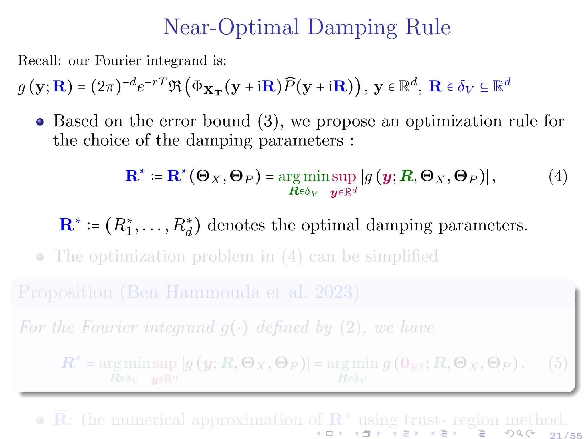
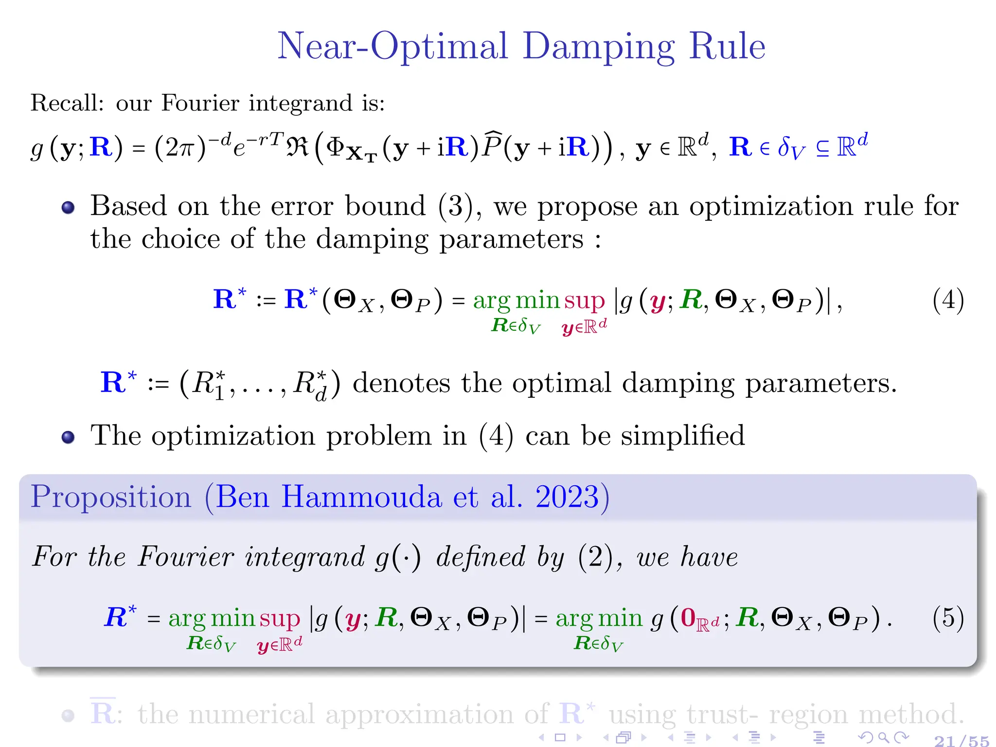
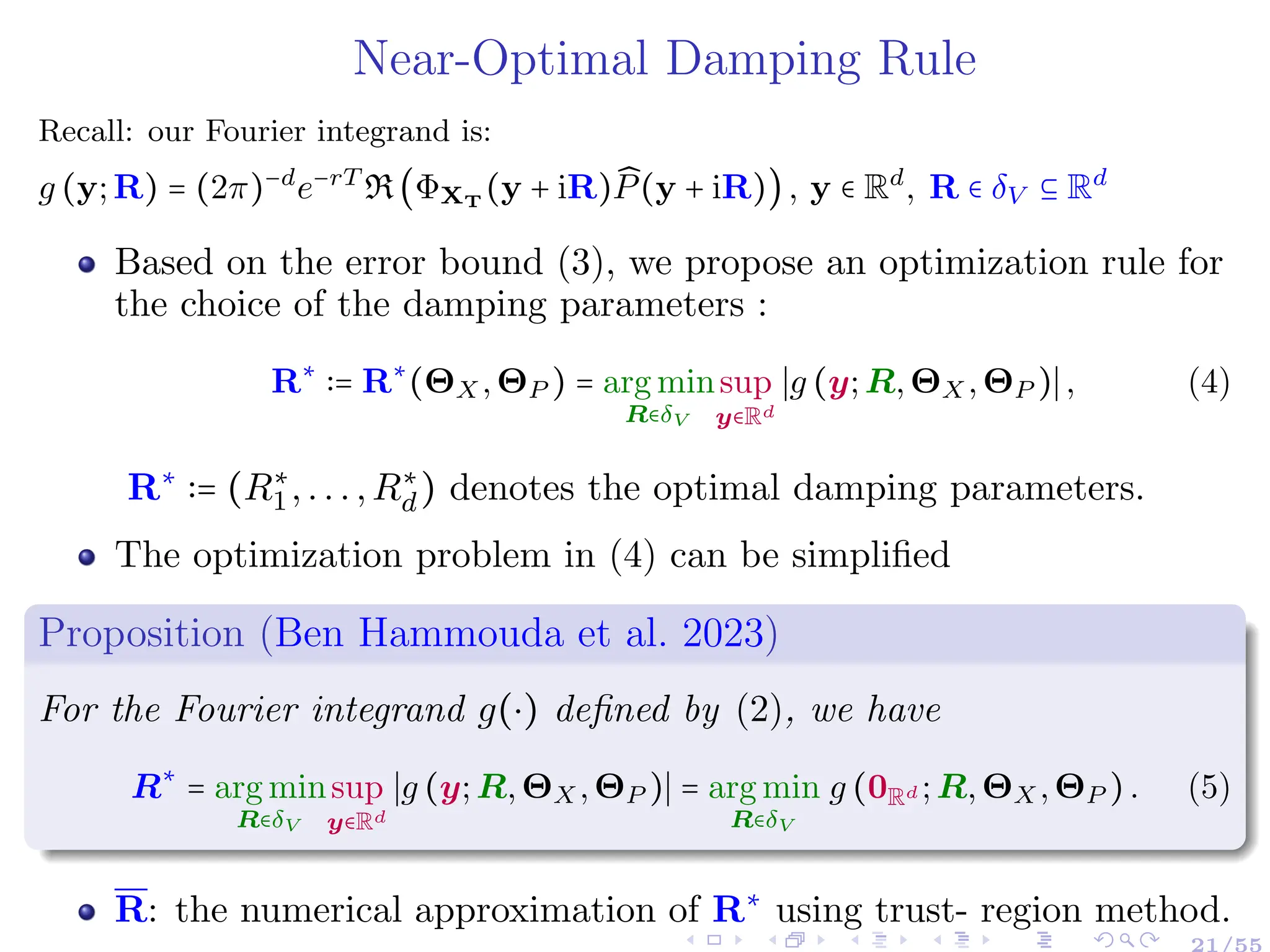
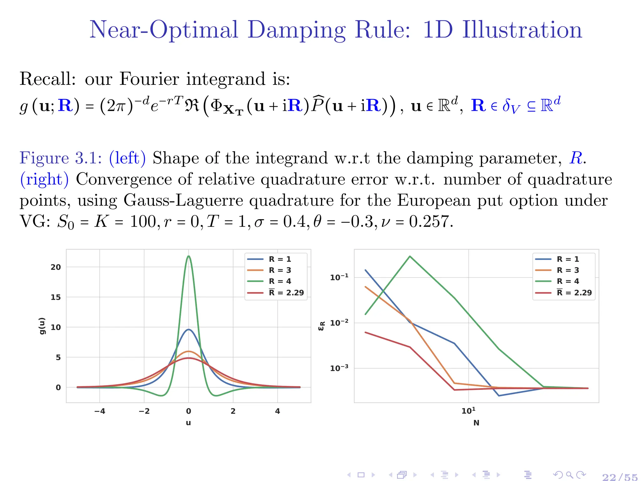
![Option value on d stocks
(Multivariate Expectation of Interest)
Recall: our Fourier integrand is:
g (y;R) = (2π)−d
e−rT
R(ΦXT
(y + iR) ̂
P(y + iR)), y ∈ Rd
, R ∈ δV ⊆ Rd
Physical space:
E[P(X(T))] =
∫Rd P(x) ρXT
(x) dx
A non-smooth
d-dimensional
integration problem
Fourier space:
∫Rd g (y;R)dy
A highly-smooth
d-dimensional
integration problem
Fourier Mapping
+ Damping Rule](https://image.slidesharecdn.com/22slidesbenhamouda-250123205348-1bb4dd63/75/Empowering-Fourier-based-Pricing-Methods-for-Efficient-Valuation-of-High-Dimensional-Derivatives-29-2048.jpg)
![Quadrature Methods: Illustration of Grids Construction
Figure 3.3: N = 81 Clenshaw-Curtis quadrature points on [0,1]2
for (left) TP,
(center) sparse grids, (right) adaptive sparse grids quadrature
(ASGQ). The ASGQ is built for the function: f(u1,u2) = 1
u2
1+exp(10 u2)+0.3
0 0.2 0.4 0.6 0.8 1
u1
0
0.1
0.2
0.3
0.4
0.5
0.6
0.7
0.8
0.9
1
u2
0 0.2 0.4 0.6 0.8 1
u1
0
0.1
0.2
0.3
0.4
0.5
0.6
0.7
0.8
0.9
1
u2
0 0.2 0.4 0.6 0.8 1
u1
0
0.1
0.2
0.3
0.4
0.5
0.6
0.7
0.8
0.9
1
u2
25/55](https://image.slidesharecdn.com/22slidesbenhamouda-250123205348-1bb4dd63/75/Empowering-Fourier-based-Pricing-Methods-for-Efficient-Valuation-of-High-Dimensional-Derivatives-32-2048.jpg)
![Quadrature Methods
Naive Quadrature operator based on a Cartesian quadrature grid
∫
Rd
g(x)ρ(x)dx ≈
d
⊗
k=1
QNk
k [g] ∶=
N1
∑
i1=1
⋯
Nd
∑
id=1
wi1 ⋯wid
g (xi1 ,...,xid
)
" Caveat: Curse of dimension: i.e., total number of quadrature
points N = ∏d
k=1 Nk.
Solution:
1 Sparsification of the grid points to reduce computational work.
2 Dimension-adaptivity to detect important dimensions of the
integrand.
Notation:
{xik
,wik
}Nk
ik=1 are respectively the sets of quadrature points and
corresponding quadrature weights for the kth dimension, 1 ≤ k ≤ d.
QNk
k [.]: the univariate quadrature operator for the kth dimension.
26/55](https://image.slidesharecdn.com/22slidesbenhamouda-250123205348-1bb4dd63/75/Empowering-Fourier-based-Pricing-Methods-for-Efficient-Valuation-of-High-Dimensional-Derivatives-33-2048.jpg)
![1D Hierarchical Construction of Quadrature Methods
Let m(⋅) ∶ N+ → N+ be a strictly increasing function with m(1) = 1;
▸ β ∈ N+: hierarchical quadrature level.
▸ m(β) ∈ N+: number of quadrature points used at level β.
Hierarchical construction: example for level 3 quadrature Qm(3)
[g]:
Qm(3)
[g] = Qm(1)
´¹¹¹¹¹¸¹¹¹¹¹
∆m(1)
[g] + (Qm(2)
− Qm(1)
´¹¹¹¹¹¹¹¹¹¹¹¹¹¹¹¹¹¹¹¹¹¹¹¹¹¹¹¹¹¹¹¹¹¹¹¹¹¹¸¹¹¹¹¹¹¹¹¹¹¹¹¹¹¹¹¹¹¹¹¹¹¹¹¹¹¹¹¹¹¹¹¹¹¹¹¹
∆m(2)
)[g] + (Qm(3)
− Qm(2)
´¹¹¹¹¹¹¹¹¹¹¹¹¹¹¹¹¹¹¹¹¹¹¹¹¹¹¹¹¹¹¹¹¹¹¹¹¹¹¸¹¹¹¹¹¹¹¹¹¹¹¹¹¹¹¹¹¹¹¹¹¹¹¹¹¹¹¹¹¹¹¹¹¹¹¹¹
∆m(3)
)[g],
where ∆m(β)
∶= Qm(β)
− Qm(β−1)
, Qm(0)
= 0: univariate detail operator.
The exact value of the integral can be written as a series expansion of
detail operators
∫
R
g(x)dx =
∞
∑
β=1
∆m(β)
[g],
27/55](https://image.slidesharecdn.com/22slidesbenhamouda-250123205348-1bb4dd63/75/Empowering-Fourier-based-Pricing-Methods-for-Efficient-Valuation-of-High-Dimensional-Derivatives-34-2048.jpg)
![Hierarchical Sparse grids: Construction
Let β = [β1,...,βd] ∈ Nd
+, m(β) ∶ N+ → N+ an increasing function,
1 1D quadrature operators: Q
m(βk)
k on m(βk) points, 1 ≤ k ≤ d.
2 Detail operator: ∆
m(βk)
k = Q
m(βk)
k − Q
m(βk−1)
k , Q
m(0)
k = 0.
3 Hierarchical surplus: ∆m(β)
= ⊗d
k=1 ∆
m(βk)
k .
4 Hierarchical sparse grid approximation: on an index set I ⊂ Nd
QI
d [g] = ∑
β∈I
∆m(β)
[g] (6)
28/55](https://image.slidesharecdn.com/22slidesbenhamouda-250123205348-1bb4dd63/75/Empowering-Fourier-based-Pricing-Methods-for-Efficient-Valuation-of-High-Dimensional-Derivatives-35-2048.jpg)
![Grids Construction
Tensor Product (TP) approach: I ∶= Iℓ = {∣∣ β ∣∣∞≤ ℓ; β ∈ Nd
+}.
Regular sparse grids (SG): I ∶ Iℓ = {∣∣ β ∣∣1≤ ℓ + d − 1; β ∈ Nd
+}
Adaptive sparse grids (ASG): Adaptive and a posteriori
construction of I = IASGQ
by profit rule
IASGQ
= {β ∈ Nd
+ ∶ Pβ ≥ T}, with Pβ =
∣∆Eβ∣
∆Wβ
:
▸ ∆Eβ = ∣Q
I∪{β}
d [g] − QI
d [g]∣ (error contribution);
▸ ∆Wβ = Work[Q
I∪{β}
d [g]] − Work[QI
d [g]] (work contribution).
Figure 3.4: 2-D Illustration (Chen 2018): Admissible index sets I (top) and
corresponding quadrature points (bottom). Left: TP; middle: SG; right: ASG .
29/55](https://image.slidesharecdn.com/22slidesbenhamouda-250123205348-1bb4dd63/75/Empowering-Fourier-based-Pricing-Methods-for-Efficient-Valuation-of-High-Dimensional-Derivatives-36-2048.jpg)
![Quasi Monte Carlo methods and Discrepancy
Let P = {ξ1,...ξM } be a set of points ξi ∈ [0,1]N
and f ∶ [0,1]N
→ R a
continuous function. A Quasi Monte Carlo (QMC) method to
approximate IN (f) = ∫[0,1]N f(y)dy is an equal weight cubature
formula of the form
IN,M (f) =
1
M
M
∑
i=1
f(ξi) .
The key concept in the analysis of QMC methods is the one of
discrepancy. Notation: for x ∈ [0,1]N
let
[0,x] ∶= [0,x1] × ... × [0,xN ]. Then
V ol([0,x]) ≈ ̂
V olP ([0,x]) ∶=
# points in [0,x]
M
for a given point set P = {ξ1,...ξM }.
Local discrepancy function ∆P ∶[0,1]N
→ [−1,1]
∆P (x) ∶= ̂
V olP ([0,x]) − V ol([0,x])
=
1
M
M
∑
i=1
1[0,x](ξi) −
N
∏
i=1
xi
000000000000000
000000000000000
000000000000000
000000000000000
000000000000000
000000000000000
000000000000000
000000000000000
000000000000000
000000000000000
000000000000000
111111111111111
111111111111111
111111111111111
111111111111111
111111111111111
111111111111111
111111111111111
111111111111111
111111111111111
111111111111111
111111111111111
x
33/55](https://image.slidesharecdn.com/22slidesbenhamouda-250123205348-1bb4dd63/75/Empowering-Fourier-based-Pricing-Methods-for-Efficient-Valuation-of-High-Dimensional-Derivatives-42-2048.jpg)
![Quasi-Monte Carlo (QMC):
Need for Domain Transformation
Recall: our Fourier integrand is:
g (y;R) = (2π)−d
e−rT
R(ΦXT
(y + iR) ̂
P(y + iR)), y ∈ Rd
, R ∈ δV ⊂ Rd
Our Fourier integrand is in Rd
BUT QMC constructions are restricted
to the generation of low-discrepancy point sets on [0,1]d
.
0 0.2 0.4 0.6 0.8 1
u1
0
0.1
0.2
0.3
0.4
0.5
0.6
0.7
0.8
0.9
1
u2
Figure 4.1: shifted QMC (Lattice rule) low discrepancy points (LDP)
in 2D
⇒ Need to transform the integration domain
34/55](https://image.slidesharecdn.com/22slidesbenhamouda-250123205348-1bb4dd63/75/Empowering-Fourier-based-Pricing-Methods-for-Efficient-Valuation-of-High-Dimensional-Derivatives-43-2048.jpg)
![Quasi-Monte Carlo (QMC):
Need for Domain Transformation
Recall: our Fourier integrand is:
g (y;R) = (2π)−d
e−rT
R(ΦXT
(y + iR) ̂
P(y + iR)), y ∈ Rd
, R ∈ δV ⊂ Rd
Our Fourier integrand is in Rd
BUT QMC constructions are restricted
to the generation of low-discrepancy point sets on [0,1]d
.
⇒ Need to transform the integration domain
Compositing with inverse cumulative distribution function, we obtain
∫
Rd
g(y)dy = ∫
[0,1]d
g ○ Ψ−1
(u;Λ)
ψ ○ Ψ−1(u;Λ)
´¹¹¹¹¹¹¹¹¹¹¹¹¹¹¹¹¹¹¹¹¹¹¹¹¹¹¹¹¹¹¹¹¹¹¹¹¹¹¸¹¹¹¹¹¹¹¹¹¹¹¹¹¹¹¹¹¹¹¹¹¹¹¹¹¹¹¹¹¹¹¹¹¹¹¹¹
=∶g̃(u;Λ)
du.
▸ ψ(⋅;Λ): a probability density function (PDF) with parameters Λ.
▸ Ψ(⋅;Λ): the cumulative distribution function (CDF) corresponding
to ψ(⋅;Λ).
34/55](https://image.slidesharecdn.com/22slidesbenhamouda-250123205348-1bb4dd63/75/Empowering-Fourier-based-Pricing-Methods-for-Efficient-Valuation-of-High-Dimensional-Derivatives-44-2048.jpg)
![Randomized Quasi-Monte Carlo (RQMC)
The transformed integration problem reads now:
∫
[0,1]d
g ○ Ψ−1
(u;Λ)
ψ ○ Ψ−1(u;Λ)
´¹¹¹¹¹¹¹¹¹¹¹¹¹¹¹¹¹¹¹¹¹¹¹¹¹¹¹¹¹¹¹¹¹¹¹¹¸¹¹¹¹¹¹¹¹¹¹¹¹¹¹¹¹¹¹¹¹¹¹¹¹¹¹¹¹¹¹¹¹¹¹¹¹¹
=∶g̃(u;Λ)
du. (7)
Once the choice of ψ(⋅;Λ) (respectively Ψ−1
(⋅;Λ)) is determined,
the RQMC estimator of (7) can be expressed as follows:
QRQMC
N,S [g̃] ∶=
1
S
S
∑
i=1
1
N
N
∑
n=1
g̃ (u(s)
n ;Λ), (8)
▸ {un}N
n=1 is the sequence of deterministic QMC points in [0,1]d
▸ For n = 1,...,N, {u
(s)
n }S
s=1: obtained by an appropriate
randomization of {un}N
n=1, e.g.,
u
(s)
n = {un + ηs}, with {ηs}S
s=1
i.i.d
∼ U([0,1]d
) and {⋅} is the
modulo-1 operator.
35/55](https://image.slidesharecdn.com/22slidesbenhamouda-250123205348-1bb4dd63/75/Empowering-Fourier-based-Pricing-Methods-for-Efficient-Valuation-of-High-Dimensional-Derivatives-45-2048.jpg)
![Previous literature (Kuo et al. 2011; Nichols et al. 2014; Ouyang et al.
2023) considers a different setting (more straightforward) for QMC:
Transformation for a weighted integration problem
(i.e., ∫Rd g(y) ρ(y) dy),
In the physical space
Assumes an independence structure
Our Setting
Recall the transformed integration problem in the Fourier space
∫
[0,1]d
g ○ Ψ−1
(u;Λ)
ψ ○ Ψ−1(u;Λ)
´¹¹¹¹¹¹¹¹¹¹¹¹¹¹¹¹¹¹¹¹¹¹¹¹¹¹¹¹¹¹¹¹¹¹¹¹¹¹¸¹¹¹¹¹¹¹¹¹¹¹¹¹¹¹¹¹¹¹¹¹¹¹¹¹¹¹¹¹¹¹¹¹¹¹¹¹
=∶g̃(u;Λ)
du.
⇒ We need to design a transformation adapted to our setting and take
into account possible dependencies between the dimensions (i.e.,
correlation between asset prices). 36/55](https://image.slidesharecdn.com/22slidesbenhamouda-250123205348-1bb4dd63/75/Empowering-Fourier-based-Pricing-Methods-for-Efficient-Valuation-of-High-Dimensional-Derivatives-46-2048.jpg)
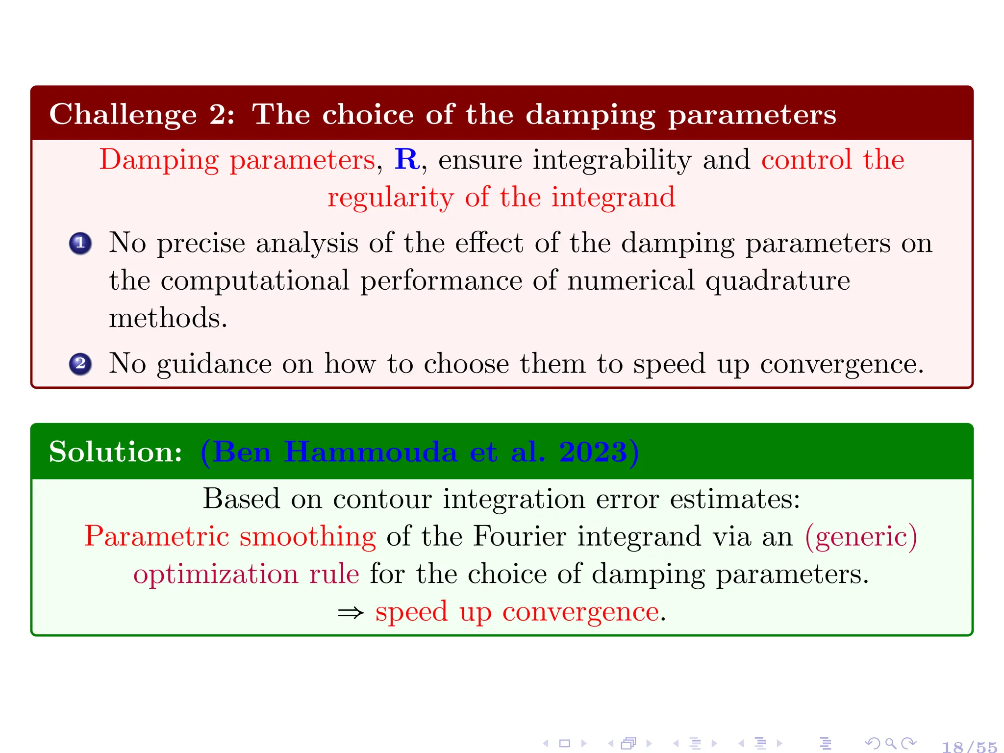
![Challenge 4: Deterioration of QMC convergence if ψ
or/and Λ are badly chosen
Observe: The denominator of g̃(u) =
g○Ψ−1(u;Λ)
ψ○Ψ−1(u;Λ)
decays to 0 as
uj → 0,1 for j = 1,...,d.
The transformed integrand may have singularities near the
boundary of [0,1]d
⇒ Deterioration of QMC convergence.
−20 −15 −10 −5 0 5 10 15 20
u
0.0
0.2
0.4
0.6
0.8
g
(
u
)
(a) Original Fourier integrand
for call option under GBM
0.0 0.2 0.4 0.6 0.8 1.0
u
0
10
20
30
40
50
60
70
̃
g
(
u
)
̃ ̃
σ = 1.0
̃ ̃
σ = 5.0
̃ ̃
σ = 9.0
(b) Transformed integrand, based
on Gaussian density with scale σ̃.
Questions
Q1: Which density to choose? Q2: How to choose its parameters?](https://image.slidesharecdn.com/22slidesbenhamouda-250123205348-1bb4dd63/75/Empowering-Fourier-based-Pricing-Methods-for-Efficient-Valuation-of-High-Dimensional-Derivatives-47-2048.jpg)
![Challenge 4: Deterioration of QMC convergence if ψ
or/and Λ are badly chosen
Observe: The denominator of g̃(u) =
g○Ψ−1(u;Λ)
ψ○Ψ−1(u;Λ)
decays to 0 as
uj → 0,1 for j = 1,...,d.
The transformed integrand may have singularities near the
boundary of [0,1]d
⇒ Deterioration of QMC convergence.
−20 −15 −10 −5 0 5 10 15 20
u
0.0
0.2
0.4
0.6
0.8
g
(
u
)
(a) Original Fourier integrand
for call option under GBM
0.0 0.2 0.4 0.6 0.8 1.0
u
0
10
20
30
40
50
60
70
̃
g
(
u
)
̃ ̃
σ = 1.0
̃ ̃
σ = 5.0
̃ ̃
σ = 9.0
(b) Transformed integrand, based
on Gaussian density with scale σ̃.
Questions
Q1: Which density to choose? Q2: How to choose its parameters?](https://image.slidesharecdn.com/22slidesbenhamouda-250123205348-1bb4dd63/75/Empowering-Fourier-based-Pricing-Methods-for-Efficient-Valuation-of-High-Dimensional-Derivatives-48-2048.jpg)
![How to choose ψ(⋅;Λ) (respectively Ψ−1(⋅;Λ) ) and
and its parameters, Λ?
For u ∈ [0,1]d
,R ∈ δV ⊂ Rd
, the transformed Fourier integrand reads:
g̃(u) =
g ○ Ψ−1
(u;Λ)
ψ ○ Ψ−1(u;Λ)
=
e−rT
(2π)d
R
⎡
⎢
⎢
⎢
⎣
̂
P(Ψ−1
(u) + iR)
ΦXT
(Ψ−1
(u) + iR)
ψ (Ψ−1(u))
⎤
⎥
⎥
⎥
⎦
.
⇒ Sufficient to design the domain transformation to control the growth
at the boundaries of the term
ΦXT
(Ψ−1(u)+iR)
ψ(Ψ−1(u))
(Conservative choice).
The payoff Fourier transforms ( ̂
P(⋅)) decay at a polynomial rate.
PDFs of the pricing models (light and semi-heavy tailed models), if
they exist, are much smoother than the payoff ⇒ the decay of their
Fourier transforms (charactersitic functions) is faster the one of the
payoff Fourier transform (Trefethen 1996; Cont et al. 2003).](https://image.slidesharecdn.com/22slidesbenhamouda-250123205348-1bb4dd63/75/Empowering-Fourier-based-Pricing-Methods-for-Efficient-Valuation-of-High-Dimensional-Derivatives-49-2048.jpg)
![How to choose ψ(⋅;Λ) (respectively Ψ−1(⋅;Λ) ) and
and its parameters, Λ?
For u ∈ [0,1]d
,R ∈ δV ⊂ Rd
, the transformed Fourier integrand reads:
g̃(u) =
g ○ Ψ−1
(u;Λ)
ψ ○ Ψ−1(u;Λ)
=
e−rT
(2π)d
R
⎡
⎢
⎢
⎢
⎣
̂
P(Ψ−1
(u) + iR)
ΦXT
(Ψ−1
(u) + iR)
ψ (Ψ−1(u))
⎤
⎥
⎥
⎥
⎦
.
⇒ Sufficient to design the domain transformation to control the growth
at the boundaries of the term
ΦXT
(Ψ−1(u)+iR)
ψ(Ψ−1(u))
(Conservative choice).
The payoff Fourier transforms ( ̂
P(⋅)) decay at a polynomial rate.
PDFs of the pricing models (light and semi-heavy tailed models), if
they exist, are much smoother than the payoff ⇒ the decay of their
Fourier transforms (charactersitic functions) is faster the one of the
payoff Fourier transform (Trefethen 1996; Cont et al. 2003).](https://image.slidesharecdn.com/22slidesbenhamouda-250123205348-1bb4dd63/75/Empowering-Fourier-based-Pricing-Methods-for-Efficient-Valuation-of-High-Dimensional-Derivatives-50-2048.jpg)
![Model-dependent Domain Transformation
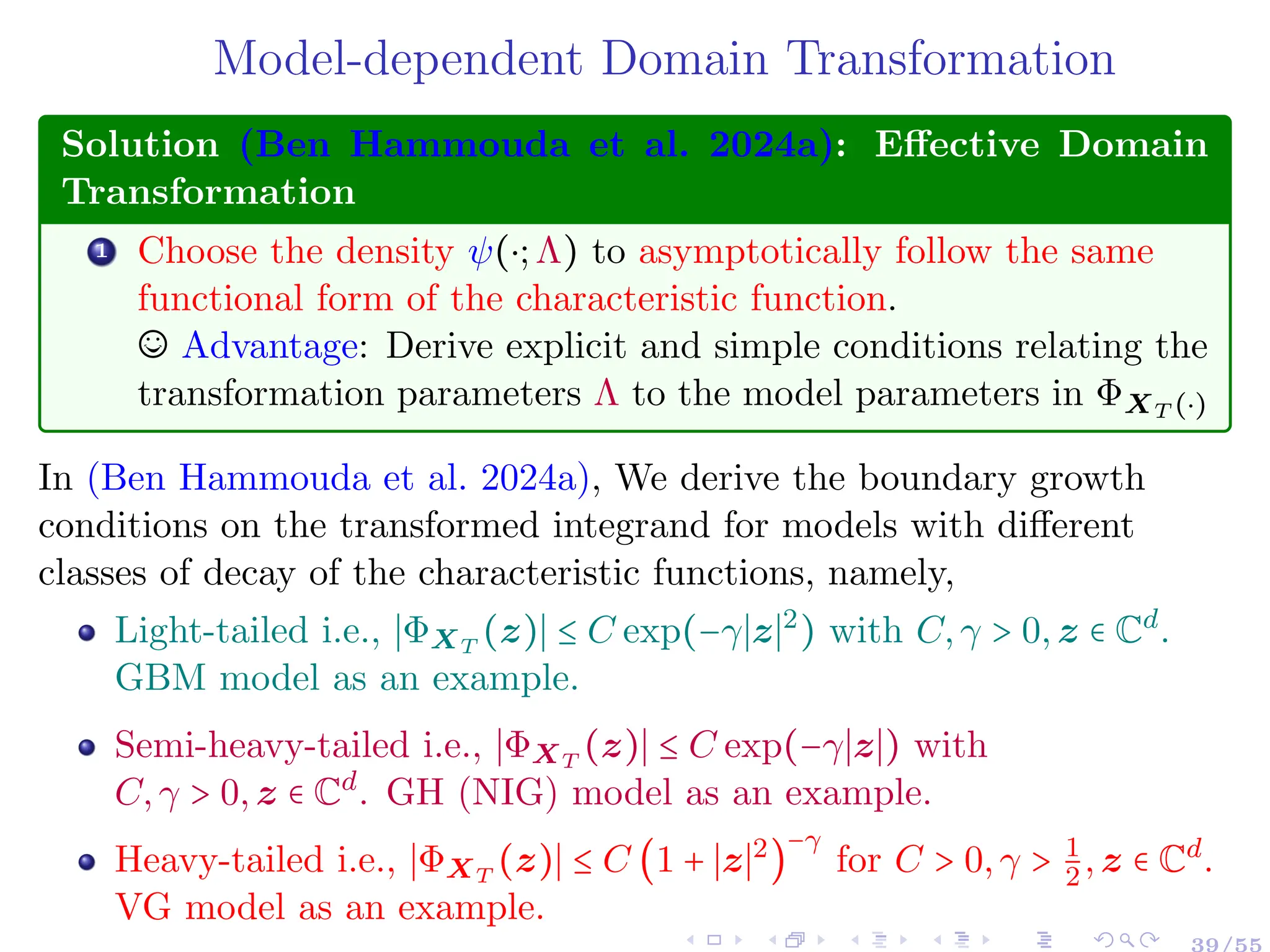
Solution (Ben Hammouda et al. 2024a): Effective Domain Transformation
1 Choose the density ψ(⋅;Λ) to asymptotically follow the same functional form of the
characteristic function.
© Advantage: Derive explicit and simple conditions relating the transformation parameters Λ
to the model parameters in ΦXT (⋅)
Table 6: Extended characteristic function: ΦXT
(z) = exp(iz′
X0)exp(iz′
µT)ϕXT
(z), and choice of ψ(⋅).
ϕXT
(z),z ∈ Cd
, I[z] ∈ δX ψ(y;Λ),y ∈ Rd
Gaussian (Λ = Σ̃):
GBM model: exp(−T
2
z′
Σz)
(2π)− d
2 (det(Σ̃))− 1
2 exp(−1
2
(y′
Σ̃
−1
y))
Generalized Student’s t (Λ = (ν̃,Σ̃)):
VG model: (1 − iνz′
θ + 1
2
νz′
Σz)
−T /ν Γ( ν̃+d
2
)(det(Σ̃))− 1
2
Γ( ν̃
2
)ν̃
d
2 π
d
2
(1 + 1
ν̃
(y′
Σ̃y))
− ν̃+d
2
NIG model: Laplace (Λ = Σ̃) and (v = 2−d
2
):
exp(δT (
√
α2 − β′
∆β −
√
α2 − (β + iz)′∆(β + iz)))
(2π)− d
2 (det(Σ̃))− 1
2 (y′
Σ̃
−1
y
2
)
v
2
Kv (
√
2y′Σ̃
−1
y)
Notation:
Σ: Covariance matrix for the Geometric Brownian Motion (GBM) model.
ν, θ, σ, Σ: Variance Gamma (VG) model parameters.
α, β, δ, ∆: Normal Inverse Gaussian (NIG) model parameters.
µ is the martingale correction term.
Kv(⋅): the modified Bessel function of the second kind.
40/55](https://image.slidesharecdn.com/22slidesbenhamouda-250123205348-1bb4dd63/75/Empowering-Fourier-based-Pricing-Methods-for-Efficient-Valuation-of-High-Dimensional-Derivatives-52-2048.jpg)
![Model-dependent Domain Transformation:
Case of Independent Assets
Using independence: Observe
ϕXT
(Ψ−1
(u)+iR)
ψ(Ψ−1(u))
= ∏
d
j=1
ϕ
X
j
T
(Ψ−1
(uj )+iRj )
ψj (Ψ−1(uj ))
Solution (Ben Hammouda et al. 2024a): Effective Domain Transformation
1 Choose the density ψ(⋅;Λ) in the change of variable to asymptotically follow the same functional
form of the extended characteristic function.
2 Select the parameters Λ to control the growth of the integrand near the boundary of [0,1]d
i.e
limuj →0,1 g̃(uj) < ∞, j = 1,...,d.
Table 7: Choice of ψ(u;Λ) ∶= ∏
d
j=1 ψj(uj;Λ) and conditions on Λ for GBM, (ii) VG and (iii) NIG. See
(Ben Hammouda et al. 2024a) for the derivation.
Model ψj(yj;Λ) Growth condition on Λ
GBM
1
√
2σ̃j
2
exp(−
y2
j
2σ̃j
2 ) (Gaussian) σ̃j ≥ 1
√
T σj
VG
Γ( ν̃+1
2
)
√
ν̃πσ̃j Γ( ν̃
2
)
(1 +
y2
j
ν̃σ̃j
2 )
−(ν̃+1)/2
(t-Student) ν̃ ≤ 2T
ν
− 1,
σ̃j = (
νσ2
j ν̃
2
)
T
ν−2T
(ν̃)
ν
4T −2ν
NIG, GH
exp(−
∣yj ∣
σ̃j
)
2σ̃j
(Laplace) σ̃j ≥ 1
δT
" In case of equality conditions, the integrand still decays at the speed of the payoff transform.](https://image.slidesharecdn.com/22slidesbenhamouda-250123205348-1bb4dd63/75/Empowering-Fourier-based-Pricing-Methods-for-Efficient-Valuation-of-High-Dimensional-Derivatives-53-2048.jpg)
![Boundary Growth Conditions: GBM as Illustration
Consider the case of independent assets, s.t. the characteristic function can be
written as
ϕXT
(u) =
d
∏
j=1
ϕXj
T
(uj),u ∈ Rd
,
where
ϕXj
T
(uj) = exp(rT − i
σj
2
T
2
uj −
σj
2
T
2
u2
j )
For the domain transformation density, we propose ψ(u) = ∏
d
j=1 ψj(uj), with
ψj(uj) =
exp(−
u2
j
2σ̃2
j
)
√
2σ̃2
j
,uj ∈ R.
⇒ The transformed integrand can be written as (y ∈ [0,1]d
)
g̃(y) ∶= (2π)−d
e−rT
e−⟨R,X0⟩
R
⎡
⎢
⎢
⎢
⎢
⎣
ei⟨Ψ−1
(y),X0⟩ ̂
P (Ψ−1
(y) + iR)
d
∏
j=1
ϕXj
T
(Ψ−1
(yj) + iRj)
ψj(Ψ−1(yj))
⎤
⎥
⎥
⎥
⎥
⎦
.
42/55](https://image.slidesharecdn.com/22slidesbenhamouda-250123205348-1bb4dd63/75/Empowering-Fourier-based-Pricing-Methods-for-Efficient-Valuation-of-High-Dimensional-Derivatives-54-2048.jpg)
![Boundary Growth Condition: GBM
The term controlling the growth of the integrand near the boundary is
rj(yj) ∶=
ϕXj
T
(Ψ−1
(yj) + iRj)
ψj(Ψ−1(yj))
, yj ∈ [0,1]. (9)
After some simplifications (9) reduces to
rj(yj) = σ̃j exp(−(Ψ−1
(yj))2
(
Tσ2
j
2
−
1
2σ̃2
j
))
´¹¹¹¹¹¹¹¹¹¹¹¹¹¹¹¹¹¹¹¹¹¹¹¹¹¹¹¹¹¹¹¹¹¹¹¹¹¹¹¹¹¹¹¹¹¹¹¹¹¹¹¹¹¹¹¹¹¹¹¹¹¹¹¹¹¹¹¹¹¹¹¹¹¹¹¹¹¹¹¹¹¹¹¹¹¹¹¹¹¹¹¹¹¹¹¹¹¹¹¹¹¹¹¹¹¹¹¹¹¹¹¹¹¹¹¹¹¸¹¹¹¹¹¹¹¹¹¹¹¹¹¹¹¹¹¹¹¹¹¹¹¹¹¹¹¹¹¹¹¹¹¹¹¹¹¹¹¹¹¹¹¹¹¹¹¹¹¹¹¹¹¹¹¹¹¹¹¹¹¹¹¹¹¹¹¹¹¹¹¹¹¹¹¹¹¹¹¹¹¹¹¹¹¹¹¹¹¹¹¹¹¹¹¹¹¹¹¹¹¹¹¹¹¹¹¹¹¹¹¹¹¹¹¹¹
∶=T1(controls the growth of the integrand near the boundary)
×
√
2π exp(−iTΨ−1
(yj)(
σ2
j
2
+ σ2
j Rj) + R2
j Tσ2
j + rT)
´¹¹¹¹¹¹¹¹¹¹¹¹¹¹¹¹¹¹¹¹¹¹¹¹¹¹¹¹¹¹¹¹¹¹¹¹¹¹¹¹¹¹¹¹¹¹¹¹¹¹¹¹¹¹¹¹¹¹¹¹¹¹¹¹¹¹¹¹¹¹¹¹¹¹¹¹¹¹¹¹¹¹¹¹¹¹¹¹¹¹¹¹¹¹¹¹¹¹¹¹¹¹¹¹¹¹¹¹¹¹¹¹¹¹¹¹¹¹¹¹¹¹¹¹¹¹¹¹¹¹¹¹¹¹¹¹¹¹¹¹¹¹¹¹¹¹¹¹¹¹¹¹¹¹¹¹¹¹¹¹¹¹¹¹¹¹¹¹¹¹¹¹¹¹¹¹¹¸¹¹¹¹¹¹¹¹¹¹¹¹¹¹¹¹¹¹¹¹¹¹¹¹¹¹¹¹¹¹¹¹¹¹¹¹¹¹¹¹¹¹¹¹¹¹¹¹¹¹¹¹¹¹¹¹¹¹¹¹¹¹¹¹¹¹¹¹¹¹¹¹¹¹¹¹¹¹¹¹¹¹¹¹¹¹¹¹¹¹¹¹¹¹¹¹¹¹¹¹¹¹¹¹¹¹¹¹¹¹¹¹¹¹¹¹¹¹¹¹¹¹¹¹¹¹¹¹¹¹¹¹¹¹¹¹¹¹¹¹¹¹¹¹¹¹¹¹¹¹¹¹¹¹¹¹¹¹¹¹¹¹¹¹¹¹¹¹¹¹¹¹¹¹¹¹
∶=T2 (bounded)
,
If we set σ̃j ≥ 1
√
T σj
⇒ T1 < ∞ as yj → 0,1 (since (Ψ−1
(yj))2
→ +∞).
43/55](https://image.slidesharecdn.com/22slidesbenhamouda-250123205348-1bb4dd63/75/Empowering-Fourier-based-Pricing-Methods-for-Efficient-Valuation-of-High-Dimensional-Derivatives-55-2048.jpg)
![Evaluation of Ψ−1
Distribution of ΨY belongs to the class of (centered) normal
mean-variance mixtures i.e. Y
d
=
√
WL ⋅ Z, with Z ∼ N(0,Id)
independent of W, and L ∈ Rd×d
(a Cholesky factor).
Applying an affine transformation in the integration yields (see
(Ben Hammouda et al. 2024a) for the proofs):
∫
[0,1]d
g (Ψ−1
Y (u))
ψY (Ψ−1
Y (u))
du = ∫
[0,1]d+1
g (Ψ−1
√
W
(ud+1)LΨ−1
Z (u−(d+1)))
ψY (Ψ−1
√
W
(ud+1)LΨ−1
Z (u−(d+1)))
du, (10)
with u−(d+1) denotes the vector excluding the (d + 1)-th
component.
(10) can be computed using QMC with (d + 1)-dimensional LDPs.
For the multivariate t-student distribution:
√
W follows the
inverse chi distribution with degrees of freedom ν̃.
For the multivariate Laplace distribution:
√
W follows the
Rayleigh distribution with scale 1
√
2
.
48/55](https://image.slidesharecdn.com/22slidesbenhamouda-250123205348-1bb4dd63/75/Empowering-Fourier-based-Pricing-Methods-for-Efficient-Valuation-of-High-Dimensional-Derivatives-61-2048.jpg)
![Model-dependent Domain Transformation:
Case of Correlated Assets
Solution (Ben Hammouda et al. 2024a): Effective Domain Transformation
1 Choose the density ψ(⋅;Λ) in the change of variable to asymptotically follow the
same functional form of the extended characteristic function.
2 Select the parameters Λ to control the growth of the integrand near the boundary
of [0,1]d
i.e limuj→0,1 g̃(uj) < ∞,j = 1,...,d.
Table 8: Choice of ψ(u;Λ) ∶= ∏
d
j=1 ψj(uj;Λ) and sufficient conditions on Λ for GBM, (ii) VG and
(iii) NIG. See (Ben Hammouda et al. 2024a) for the derivation. Kλ(y) is the modified Bessel
function of the second kind with λ = 2−d
2
, y > 0. ” ⪰ 0” ∶ denotes positive-semidefiniteness of a
matrix
Model ψ(y;Λ) Growth condition on Λ
GBM Gaussian: (2π)− d
2 (det(Σ̃))− 1
2 exp(−1
2(y′
Σ̃
−1
y)) TΣ − Σ̃
−1
⪰ 0
VG Generalized Student’s t:
Γ(ν̃+d
2
)(det(Σ̃))− 1
2
Γ(ν̃
2
)ν̃
d
2 π
d
2
(1 + 1
ν̃
(y′
Σ̃y))
− ν̃+d
2
ν̃ = 2T
ν −d, Σ−Σ̃
−1
⪰ 0
or
ν̃ ≤ 2T
ν − d, Σ̃ = Σ−1
GH Laplace: (2π)− d
2 (det(Σ̃))− 1
2 (y′Σ̃
−1
y
2 )
λ
2
Kλ (
√
2y′Σ̃
−1
y) δ2
T2
∆ − 2Σ̃
−1
⪰ 0](https://image.slidesharecdn.com/22slidesbenhamouda-250123205348-1bb4dd63/75/Empowering-Fourier-based-Pricing-Methods-for-Efficient-Valuation-of-High-Dimensional-Derivatives-62-2048.jpg)

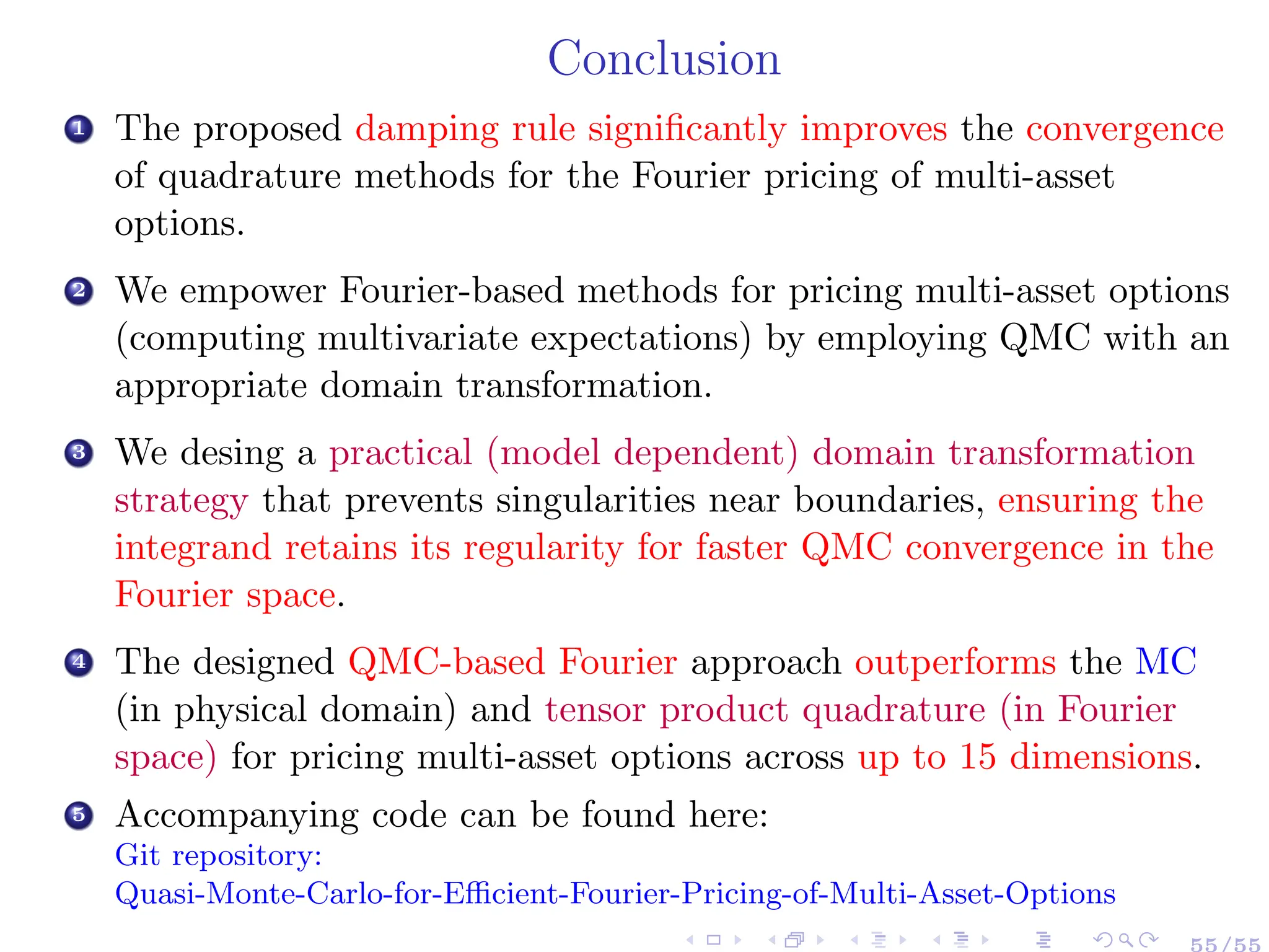
![Conclusion
Task (Option Pricing and Beyond): Efficiently compute:
E[g(X(T))] = ∫
Rd
g(x) ρXT
(x) dx.
The pdf, ρXT
, is not known explicitly or expensive to
sample from.
g(⋅) is non-smooth.
The dimension d is large.
54/55](https://image.slidesharecdn.com/22slidesbenhamouda-250123205348-1bb4dd63/75/Empowering-Fourier-based-Pricing-Methods-for-Efficient-Valuation-of-High-Dimensional-Derivatives-68-2048.jpg)
![Conclusion
Task (Option Pricing and Beyond): Efficiently compute:
E[g(X(T))] = ∫
Rd
g(x) ρXT
(x) dx.
1 Uncovering the Available Hidden Regularity:
Physical space:
∫Rd g(x) ρXT
(x) dx
Fourier space:
1
(2π)d ∫Rd ̂
g(u + iR) Φ(u + iR) du
Fourier Transform
2 Parametric Smoothing:
Challenge:
Arbitrary choices for R may deteriorate
the regularity of Fourier integrand.
Solution:
(Generic) optimization rule for the choice of R
based on contour integration error estimates.
3 Addressing the Curse of Dimension:
Challenge:
Complexity of (standard) tensor
product (TP) quadrature ↗
exponentially with the dimension, d.
Solution:
▸ Sparsification and dimension-adaptivity.
▸ Quasi-Monte Carlo (QMC) with efficient domain
transformation.
54/55](https://image.slidesharecdn.com/22slidesbenhamouda-250123205348-1bb4dd63/75/Empowering-Fourier-based-Pricing-Methods-for-Efficient-Valuation-of-High-Dimensional-Derivatives-69-2048.jpg)
![References I
[1] J.-P. Aguilar. “Some pricing tools for the Variance Gamma
model”. In: International Journal of Theoretical and Applied
Finance 23.04 (2020), p. 2050025.
[2] C. Bayer, M. Siebenmorgen, and R. Tempone. “Smoothing the
payoff for efficient computation of basket option pricing.”. In:
Quantitative Finance 18.3 (2018), pp. 491–505.
[3] C. Ben Hammouda, C. Bayer, and R. Tempone. “Hierarchical
adaptive sparse grids and quasi-Monte Carlo for option pricing
under the rough Bergomi model”. In: Quantitative Finance 20.9
(2020), pp. 1457–1473.
[4] C. Ben Hammouda, C. Bayer, and R. Tempone. “Numerical
smoothing with hierarchical adaptive sparse grids and
quasi-Monte Carlo methods for efficient option pricing”. In:
Quantitative Finance (2022), pp. 1–19.
55/55](https://image.slidesharecdn.com/22slidesbenhamouda-250123205348-1bb4dd63/75/Empowering-Fourier-based-Pricing-Methods-for-Efficient-Valuation-of-High-Dimensional-Derivatives-72-2048.jpg)
![References II
[5] C. Ben Hammouda et al. “Optimal Damping with Hierarchical
Adaptive Quadrature for Efficient Fourier Pricing of Multi-Asset
Options in Lévy Models”. In: Journal of Computational Finance
27.3 (2023), pp. 43–86.
[6] C. Ben Hammouda et al. “Quasi-Monte Carlo for Efficient
Fourier Pricing of Multi-Asset Options”. In: arXiv preprint
arXiv:2403.02832 (2024).
[7] C. Ben Hammouda, C. Bayer, and R. Tempone. “Multilevel
Monte Carlo with numerical smoothing for robust and efficient
computation of probabilities and densities”. In: SIAM Journal on
Scientific Computing 46.3 (2024), A1514–A1548.
[8] P. Carr and D. Madan. “Option valuation using the fast Fourier
transform”. In: Journal of computational finance 2.4 (1999),
pp. 61–73.
55/55](https://image.slidesharecdn.com/22slidesbenhamouda-250123205348-1bb4dd63/75/Empowering-Fourier-based-Pricing-Methods-for-Efficient-Valuation-of-High-Dimensional-Derivatives-73-2048.jpg)
![References III
[9] P. Chen. “Sparse quadrature for high-dimensional integration
with Gaussian measure”. In: ESAIM: Mathematical Modelling
and Numerical Analysis 52.2 (2018), pp. 631–657.
[10] R. Cont and P. Tankov. Financial Modelling with Jump
Processes. Chapman and Hall/CRC, 2003.
[11] P. J. Davis and P. Rabinowitz. Methods of numerical integration.
Courier Corporation, 2007.
[12] J. Dick, F. Y. Kuo, and I. H. Sloan. “High-dimensional
integration: the quasi-Monte Carlo way”. In: Acta Numerica 22
(2013), pp. 133–288.
[13] D. Duffie, D. Filipović, and W. Schachermayer. “Affine processes
and applications in finance”. In: The Annals of Applied
Probability 13.3 (2003), pp. 984–1053.
55/55](https://image.slidesharecdn.com/22slidesbenhamouda-250123205348-1bb4dd63/75/Empowering-Fourier-based-Pricing-Methods-for-Efficient-Valuation-of-High-Dimensional-Derivatives-74-2048.jpg)
![References IV
[14] E. Eberlein. “Jump–type Lévy processes”. In: Handbook of
financial time series. Springer, 2009, pp. 439–455.
[15] E. Eberlein, K. Glau, and A. Papapantoleon. “Analysis of Fourier
transform valuation formulas and applications”. In: Applied
Mathematical Finance 17.3 (2010), pp. 211–240.
[16] O. El Euch, J. Gatheral, and M. Rosenbaum. “Roughening
heston”. In: Risk (2019), pp. 84–89.
[17] O. G. Ernst, B. Sprungk, and L. Tamellini. “Convergence of
sparse collocation for functions of countably many Gaussian
random variables (with application to elliptic PDEs)”. In: SIAM
Journal on Numerical Analysis 56.2 (2018), pp. 877–905.
[18] F. Fang and C. W. Oosterlee. “A novel pricing method for
European options based on Fourier-cosine series expansions”. In:
SIAM Journal on Scientific Computing 31.2 (2009), pp. 826–848.
55/55](https://image.slidesharecdn.com/22slidesbenhamouda-250123205348-1bb4dd63/75/Empowering-Fourier-based-Pricing-Methods-for-Efficient-Valuation-of-High-Dimensional-Derivatives-75-2048.jpg)
![References V
[19] Z. He, C. Weng, and X. Wang. “Efficient computation of option
prices and Greeks by quasi–Monte Carlo method with smoothing
and dimension reduction”. In: SIAM Journal on Scientific
Computing 39.2 (2017), B298–B322.
[20] J. Healy. “The Pricing of Vanilla Options with Cash Dividends
as a Classic Vanilla Basket Option Problem”. In: arXiv preprint
arXiv:2106.12971 (2021).
[21] T. R. Hurd and Z. Zhou. “A Fourier transform method for
spread option pricing”. In: SIAM Journal on Financial
Mathematics 1.1 (2010), pp. 142–157.
[22] F. Y. Kuo, C. Schwab, and I. H. Sloan. “Quasi-Monte Carlo
methods for high-dimensional integration: the standard (weighted
Hilbert space) setting and beyond”. In: The ANZIAM Journal
53.1 (2011), pp. 1–37.
55/55](https://image.slidesharecdn.com/22slidesbenhamouda-250123205348-1bb4dd63/75/Empowering-Fourier-based-Pricing-Methods-for-Efficient-Valuation-of-High-Dimensional-Derivatives-76-2048.jpg)
![References VI
[23] F. Y. Kuo et al. “High dimensional integration of kinks and
jumps—smoothing by preintegration”. In: Journal of
Computational and Applied Mathematics 344 (2018), pp. 259–274.
[24] A. L. Lewis. “A simple option formula for general jump-diffusion
and other exponential Lévy processes”. In: Available at SSRN
282110 (2001).
[25] J. A. Nichols and F. Y. Kuo. “Fast CBC construction of
randomly shifted lattice rules achieving O (n- 1+ δ) convergence
for unbounded integrands over Rs in weighted spaces with POD
weights”. In: Journal of Complexity 30.4 (2014), pp. 444–468.
[26] D. Ouyang, X. Wang, and Z. He. “Quasi-Monte Carlo for
unbounded integrands with importance sampling”. In: arXiv
preprint arXiv:2310.00650 (2023).
55/55](https://image.slidesharecdn.com/22slidesbenhamouda-250123205348-1bb4dd63/75/Empowering-Fourier-based-Pricing-Methods-for-Efficient-Valuation-of-High-Dimensional-Derivatives-77-2048.jpg)
![References VII
[27] L. N. Trefethen. “Finite difference and spectral methods for
ordinary and partial differential equations”. In: (1996).
55/55](https://image.slidesharecdn.com/22slidesbenhamouda-250123205348-1bb4dd63/75/Empowering-Fourier-based-Pricing-Methods-for-Efficient-Valuation-of-High-Dimensional-Derivatives-78-2048.jpg)

The document discusses efficient pricing methods for high-dimensional derivatives using Fourier-based techniques. It highlights challenges such as the non-smoothness of payoff functions and large dimensions, proposing solutions like mapping to Fourier space and using quasi-Monte Carlo methods. Key findings and methodologies are summarized based on collaborative research involving multiple authors and related works.