Download to read offline


![2 Foundations
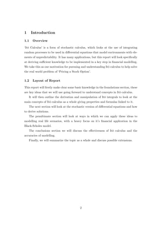
2.1 Ordinary Calculus
Standard Partitions
Definition 2.1.1. Similar to the partition in [3, Section 2.1.1], we define the standard
partition of a region [a, t] to be the split into n sub-intervals a < t1 < t2 < ... < tn−1 <
tn = t, such that the largest difference between two intervals, namely (ti+1 −ti) decreases
as n increases, written as {tn
i }, with n → ∞ ⇒ maxi=0,...,n−1(ti+1 − ti) → 0.
Riemann & Riemann-Stieltjes integrals
The formulation of (Riemann) integrals, are as such, over the interval [0, T] and xi such
that ti−1 ≤ xi ≤ ti, for f(t) shown here diagrammatically:
Figure 1: f(xi) taken for the xi in-between ti−1 and ti, the transition is shown with
more intervals to emphasise the limit to infinity, an adaptation of [3, Figure 2.1.1 p.89].
Definition 2.1.2. As from [3, p.88] for an standard partition of [0, T], {tn
i } (Def. 2.1.1)
the Riemann integral of a function f(t) with respect to t is F, the summation of the
function evaluated between the interval multiplied by the length, taken in limit where
n → ∞ such that:
F = lim
n→∞
n
i=1
f(xi)(ti − ti−1). (2.1)
If this limit exists,
F =
T
0
f(t) dt.
Which is the definition and notation of an ordinary integral we are familiar with.
3](https://image.slidesharecdn.com/3296b155-6d57-4931-bbc4-d7bce87ac5d8-150616142723-lva1-app6891/85/Stephens-L-4-320.jpg)
![However, the Riemann-Stieltjes form (as in [3, p.93]) is slightly different, where
instead of intervals of time, we are integrating with respect to a function, G(t) (why it
is useful to define this is seen in §2.3).
Definition 2.1.3. The Riemann-Stieltjes integral of a function f(t) with respect to
G(t) over the interval [0, T] with a standard partition in the form {tn
i }, is the summation
of the function f(xi) evaluated between the interval, multiplied by the change in the
function G over that interval, taken in limit where n → ∞ such that:
Fg = lim
n→∞
n
i=1
f(xi) [G(ti) − G(ti−1)] . (2.2)
Again, if this limit exists
Fg =
T
0
f(t) dG(t).
To measure the variation and quadratic variation as seen in [1, p.4,p.8] respectively, for
of a function f with a standard partition in the form {tn
i } over an interval [a, b], we
make the following definitions:
Definition 2.1.4. The variation of a f is (where the limit exists),
Vf ([a, b]) = lim
n→∞
n
i=1
|f(ti) − f(ti−1)| . (2.3)
It is the limit of the sum of the absolute value of the change in the function between
two consecutive intervals.
Definition 2.1.5. The quadratic variation of f is, (where the limit exists)
[f] (t) = lim
n→∞
n
i=1
(f(ti) − f(ti−1))2
. (2.4)
It is the limit of the sum of the change in the function between two consecutive
intervals, squared.
4](https://image.slidesharecdn.com/3296b155-6d57-4931-bbc4-d7bce87ac5d8-150616142723-lva1-app6891/85/Stephens-L-5-320.jpg)
![2.2 Discrete time models
Probability Space
Most of this section will use [6] for definitions of simple concepts in probability, needed
for going forward in this report.
We look at the concept of a probability space, assuming a basic knowledge of set
theory and using the definition on [6, p.19]:
Definition 2.2.1. A space, Ω is a set of elements ωi, called the certain event, as in,
definitely one of the elements of the set will occur. Subsets in this space are defined as
the events. The empty set, {∅} is referred to as the impossible event, as it contains no
elements of the certain event, thus making the event occurring impossible.
For example, flipping a coin with the outcome heads (h) or tails (t). The probability
space would consist of Ω = {h, t}. An event O, ‘landing on a heads’, would be O = {h}.
The event N ‘not landing on heads or tails’, being N = {∅}, is impossible because a
side has to be chosen.
2.2.1 Event fields
As from [1, p.22] we can define the information gathered at time t to be denoted by Ft.
Example 2.1. Two coin tosses:
Say we were to toss a coin twice Ci = h or t, i ∈ [1, 2] and record the order of results,
where Ω = {(C1, C2)} = {(h, h), (h, t), (t, h), (t, t)}:
Case 1. At time t = 0 we have not learnt anything yet, so the field is F0= {∅, Ω}
Case 2. At time t = 1 we have the information from the first coin flip. Denote the set
H = {(h, C2)}. Now we know that at time 1 if it was heads, set H is true, but if
it was tails, H is not true and ¯H is, so F1= ∅, Ω, H, ¯H .
Case 3. At time t = 2 we have all the information from the flips and we have all the
possible subsets of Ω, denoted by 2Ω, so F2= 2Ω .
Notice that F0 ⊂ F1 ⊂ F2 as information is not lost. A diagrammatic atomization of
this process looks like:
5](https://image.slidesharecdn.com/3296b155-6d57-4931-bbc4-d7bce87ac5d8-150616142723-lva1-app6891/85/Stephens-L-6-320.jpg)
![Figure 2: Atomization of the event field for three time values.
2.2.2 Filtrations
As from [1, p.23] we define filtrations F as a collection of the event fields of a probability
space. Taking from the fields defined in Example 2.1, F = {F0, F1, F2} would be an
example of a filtration.
2.3 General Probability
Probability Value
Definition 2.3.1. The probability value, by Kolmogoroff’s axioms [6, p.6], with
events A and B:
• The probability of an event A occurring, is the positive real number assigned by
P(A) where P(A) ≥ 0.
• An event A which is definitely to occur has the probability P(A) = 1.
• If the two events A and B are entirely independent of each other: P(A + B) =
P(A) + P(B)
If we look back to Example 2.1, with the coin being weighted so that there was a
1 in 4 chance of it landing on tails. We can measure the probability with P(ω) for all
ω ∈ Ω as such, where Ω = {(h, h), (h, t), (t, h), (t, t)}:
P(h, h) = 0.5625 P(h, t) = 0.1875 P(t, h) = 0.1875 P(t, t) = 0.0625. (2.5)
The next two sub-sections on Random Variables and Density & Distribution func-
tions are from the definitions found in [4, p.7-10], which goes more extensively into these
topics.
6](https://image.slidesharecdn.com/3296b155-6d57-4931-bbc4-d7bce87ac5d8-150616142723-lva1-app6891/85/Stephens-L-7-320.jpg)
![Random Variables
Definition 2.3.2. A random variable Y is discrete on a sample space Ω and attaches
values to the element ω such that Y (ωi) = yi ∀i ∈ [1, ..., k].
Definition 2.3.3. A random variable X is continuous on a space Ω if it has an
infinite number of possible values, the outcome can be X = x ∈ R.
Density & Distribution functions
Looking solely at continuous random variables (CRV’s) for now:
Definition 2.3.4. A probability density function (PDF) g(x) is defined for the CRV,
X = x, over the infinite range −∞ < x < ∞ where:
• 0 ≤ g(x)
• P(x1 ≤ x ≤ x2) =
x2
x1
g(x) dx
•
∞
−∞ g(x) dx = 1
Definition 2.3.5. A cumulative distribution function (CDF) G(˜x), is defined for the
CRV, X = ˜x, over the infinite range −∞ < ˜x < ∞ to be
G(˜x) = P(X ≤ ˜x) =
˜x
−∞
g(x) dx. (2.6)
Theorem 2.3.1. For a CRV X, the probability
P(x1 ≤ x ≤ x2) = G(x2) − G(x1). (2.7)
Proof. The probability x lies in the interval, by the definition of a PDF is
P(x1 ≤ x ≤ x2) =
x2
x1
g(x) dx =
x2
−∞
g(x) dx −
x1
−∞
g(x) dx,
By definition of a CDF, G(x2) =
x2
−∞ g(x) dx and G(x1) =
x1
−∞ g(x) dx.
Expectation & Variance
From [6, p.104], we get our definition of expected value, or expectation:
Definition 2.3.6. The expectation of a discrete random variable Y , for probabilities
of all events in the space, pi = P {Y = yi} is:
E(Y ) =
i
yipi.
7](https://image.slidesharecdn.com/3296b155-6d57-4931-bbc4-d7bce87ac5d8-150616142723-lva1-app6891/85/Stephens-L-8-320.jpg)
![The continuous form involves the Riemann-Stieltjes integral (§2.1), but over an in-
finite interval −∞ < x−n < x−n+1 < ... < xn−1 < xn = ∞.
Definition 2.3.7. The expectation of a continuous random variable X, where G(x)
is the cumulative distribution function of X with known derivative g(x) is:
E(X) = lim
n→∞
n
i=1
xi [G(xi) − G(xi−1)] =
∞
−∞
x dG(x) =
∞
−∞
xg(x) dx.
From [6, p.104], we get our definition of variance commonly noted as σ2, where σ is
known as the standard deviation, with identities seen in [4, p.11]:
Definition 2.3.8. The variance of a discrete random variable Y , with expectation
(or mean) E(Y ) = µ, for probabilities of all events in the space, pi = P {Y = yi} is:
σ2
Y =
i
(yi − µ)2
pi = E (Y − µ)2
= E(Y 2
) − 2E(Y )µ + µ2
= E(Y 2
) − µ2
.
The continuous form, again uses the Riemann-Stieltjes integral over an infinite in-
terval −∞ < x−n < x−n+1 < ... < xn−1 < xn = ∞ where:
Definition 2.3.9. The variance of a continuous random variable X, where G(x) is
the cumulative distribution function of X with known derivative g(x) along with
the expectation E(X) = µ is:
σ2
X = lim
n→∞
n
i=1
(xi − µ)2
[G(xi) − G(xi−1)] =
∞
−∞
(x − µ)2
dG(x) =
∞
−∞
(x − µ)2
g(x) dx.
Gaussian Normal Variable
Having defined probability density functions previously in this section, we now look at
a specific case used going forward, defined in [1, 4, p.41,p.15].
Definition 2.3.10. Gaussian normal variable (GNV), for a random variable X =
N(µ, σ2) with E(X) = µ and V ar(X) = σ2, the PDF g(x) is, for ∞ < x < ∞ :
g(x) =
1
σ
√
2π
· e
−
(x − µ)2
2σ2
.
Hence, the CDF for X = ˜x:
G(˜x) =
˜x
−∞
1
σ
√
2π
· e
−
(x − µ)2
2σ2
dx,
8](https://image.slidesharecdn.com/3296b155-6d57-4931-bbc4-d7bce87ac5d8-150616142723-lva1-app6891/85/Stephens-L-9-320.jpg)
![with:
∞
−∞
g(x) = 1
The generally used standard normal is defined in the same way but with µ = 0 and
σ2 = 1 so that:
s(z) =
1
√
2π
· e
−
z2
2 .
We can see that any normal can be linearly transformed to standard from by the fol-
lowing, with guidance from [11, S.1]:
Theorem 2.3.2. For X = N(µ, σ2) and Z = N(0, 1), we can map X → Z with the
transform Z =
X − µ
σ
Proof. x = µ + σz and dx = σdz so:
P(x1 ≤ x ≤ x2) = P(x1 ≤ µ+σz ≤ x2) =
x2
x1
1
√
2πσ
·e
−
(µ + σz − µ)2
2σ2
σdz =
x2
x1
s(z) dz.
Measurability
As from [1, p.23], for a specified F, any set inside is measurable. A discrete random
variable Y defined on Ω is F-measurable if given an event in the field has occured, then
we know which value of Y has also. If we again go back to Example 2.1, and recall
F0= {∅, Ω}, F1= ∅, Ω, H, ¯H , F2= 2Ω :
If Y1(h, h) = Y1(h, t) = 0.4 and Y1(t, h) = Y1(t, t) = 1.6, Y1 is F1-measurable as for
{ω : Y1(ω) = 0.4} = {(h, h), (h, t)} = H ∈ F1 and {ω : Y1(ω) = 1.6} = {(t, h), (t, t)} =
¯H ∈ F1.
If Y2(h, h) = 0.16 and Y2(t, h) = Y2(t, h) = 0.64, Y2(t, t) = 2.56, Y2 is F2-measurable
as for {ω : Y2(ω) = 0.64} = {(h, t), (t, h)} ∈ F2 and but not F1-measurable as
{(h, t), (t, h)} /∈ F1.
Filtered Probability Spaces
As in [1, p.50], collecting what we have previously defined, we can structure the definition
of a Filtered Probability Space being (Ω, F, F, P), for a space Ω (Definition 2.2.1) with
an event field F (Section 2.2.1) and a filtration (Section 2.2.2) and probability value P
(Definition 2.3.1).
9](https://image.slidesharecdn.com/3296b155-6d57-4931-bbc4-d7bce87ac5d8-150616142723-lva1-app6891/85/Stephens-L-10-320.jpg)
![2.3.1 Stochastic & Adapted Processes
Discrete time
As in [1, Def 2.1], a discrete time stochastic process for t ∈ [0, 1, ..., T] is the collection
of random variables {Y (t)}. If a process Y (t) is Ft-measurable for all 0 ≤ t < T, it is
known as an adapted process.
Continuous time
Continuous Stochastic processes can be seen as the limit of a discrete time process as
the time increment decreases. They are complicated to describe and require continuity
theory also involving c´adl´ag functions, rigorously detailed in [1, Section 2.8, p.47-54].
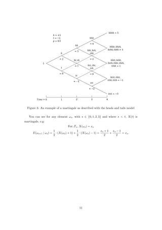
Martingales
A martingale is a process that has the same expected value for the next step as the
actual value at the previous step. More concretely defined as described in [1, p.51]:
Definition 2.3.11. For a filtered probability space (Ω, F, F, P) and s < t, if a process
has the expectation to be the same value as at the point in the process up to that we have
information for. Formally written as:
The expected value of X(t) given Fs is X(s) ⇔ E(X(t) | Fs) = X(s), (2.8)
then the process X(t) is martingale.
To give an example to help envision the concept of a martingale process, we take a
game in which the player starts with £1 and flips a fair coin. For every time it lands on
heads (h) the player is given £1, for every time it lands on tails (t), the player loses £1.
For example, if this is trialled for four flips of the coin, the following diagram shows the
outcomes:
10](https://image.slidesharecdn.com/3296b155-6d57-4931-bbc4-d7bce87ac5d8-150616142723-lva1-app6891/85/Stephens-L-11-320.jpg)
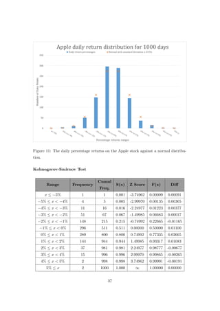
![2.4 Brownian Motion
To evaluate the cumulative effect of noise only, we can use the stochastic process first
described by R. Brown, in 1828. Starting by defining it’s properties, we will go on to
look at how it is realised and how it is used in stochastic calculus. Using [1, p.56] and
[5, p.127]:
Definition 2.4.1. Brownian motion B(t), t ∈ R>0 is:
• B(0) = x ∈ R, where x is its starting value (typically B(0) = 0 , Bx(0) = x).
• ∀n ∈ N>0, and a standard partition {tn
i } of [0, t] where i < j (i, j ∈ N>0):
B(tj)−B(ti) is an normal random variable, with distribution N(0, ti −tj).
B(tj) − B(ti) is independent of B(th) for h < i.
• B(t) is a real valued continuous function.
Using this definition, we can plot a sample path where B(0) = 0 to B(1) to give an
idea of the visual behaviour of the function.
Figure 4: Created to appear continuous using 10,000 time steps with distribution N(0, 0.0001).
12](https://image.slidesharecdn.com/3296b155-6d57-4931-bbc4-d7bce87ac5d8-150616142723-lva1-app6891/85/Stephens-L-13-320.jpg)
![Theorem 2.4.1. We see that, although continuous, Brownian motion paths have some
other properties themselves [1, p.64], almost always (there exists paths that do not
have these properties but have essentially zero likelihood of occurring). For a realisation
0 ≤ t ≤ T, the path has, with probability one:
1. No differentiability.
2. Quadratic variation t on [0, t].
3. Infinite variation on B(ti + ε) − B(ti), ∀ti 0 ≤ ti ≤ T and 0 < ε (any sized
interval).
Proof. 1. [1, p.64 Theorem 3.5]:
B(t + dt) − B(t)
dt
=
N(0, t + dt − t)
dt
=
√
dt
dt
N(0, 1) =
1
√
dt
N(0, 1) (2.9)
But we look at the limit as dt tends to zero where X = N(0, 1) and P(X = 0) = 0:
lim
dt→0
[P(
1
√
dt
|X| > K)] = 1 , ∀K ∈ R
As:
lim
A→∞
P
√
A >
K
|X|
= 1 , ∀K ∈ R, X = N(0, 1)
So the distribution in 2.9 is not finite, therefore the derivative does not exist almost
always.
Proof. 2. In the standard partition in the form {tn
i } of the interval [0, t] we look at the
expected quadratic variation
E [B] (t) = E lim
n→∞
n
i=1
(B(ti) − B(ti−1))2
= lim
n→∞
n
i=1
E (B(ti) − B(ti−1))2
,
but we see, by the definition of variance with zero mean in §2.3:
E (B(ti) − B(ti−1))2
= V ar (B(ti) − B(ti−1)) = V ar (N(0, ti − ti−1)) = ti − ti−1.
So the limit becomes:
E [B] (t) = lim
n→∞
n
i=1
ti − ti−1.
Which is a telescoping sum, resulting in:
E [B] (t) = tn − t0 = t − 0 = t.
13](https://image.slidesharecdn.com/3296b155-6d57-4931-bbc4-d7bce87ac5d8-150616142723-lva1-app6891/85/Stephens-L-14-320.jpg)
![Proof. 3. Using [10, P.1], Looking at the interval [ti, ti + ε], as ε > 0 and partitioned in
the form sm
j , using the definition of the variation of a function, equation 2.3:
VB([ti, ti + ε]) = lim
m→∞
m
j=1
|B(sj) − B(sj−1)| ≥ lim
m→∞
m
j=1
|B(sj) − B(sj−1)|2
maxj=1...m |B(sj) − B(sj−1)|
.
RHS numerator:
lim
m→∞
m
j=1
|B(sj) − B(sj−1)|2
→ t.
RHS denominator tends to zero by the definition of our standard partition (as in 2.1.1)
lim
m→∞
maxj=1...m |B(sj) − B(sj−1)| = lim
m→∞
maxj=1...m sj − sj−1 |Nj(0, 1)| → 0.
Therefore:
VB([ti, ti + ε]) → ∞.
for any finitely small ε, hence infinite variation.
Brownian Motion martingale property
It can be noted that Brownian motion is an example of a continuous martingale pro-
cesses. Due to the independence and the distribution of the intervals of Brownian
Motion, we have the result that
E(B(tj)|Fti ) = B(ti).
14](https://image.slidesharecdn.com/3296b155-6d57-4931-bbc4-d7bce87ac5d8-150616142723-lva1-app6891/85/Stephens-L-15-320.jpg)
![3 It¯o & Stochastic Calculus
3.1 Motivation
Definition 3.1.1. Riemann-Stieltjes Problem [3, p.96 Theorem 3.5], the following in-
tegral is undefined:
1
0
B(t) dB(t). (3.1)
Proof. B(ti) − B(ti−1) has infinite variation, so the limit:
FB(t) = lim
n→∞
n
i=1
B(ti) [B(ti) − B(ti−1)] .
does not exist.
So we need to define a different kind of integral that does exist for these cases, and
then go on to define a class of differential equations used for stochastic processes.
3.2 It¯o Integral
Definition & Properties
We see from our motivation, that integrating a stochastic process creates problems using
the Riemann-Stieltjes integral, hence the development and implementation of stochastic
calculus and the It¯o integral as in [2, p.2]:
Definition 3.2.1. An It¯o integral is of the form, where X and H can be stochastic
processes
X dH. (3.2)
But if we first look at this integral with respect to processes we are familiar with
and which are used traditionally, we derive a different form of the integral
T
0
X(t) dB(t). (3.3)
Where X is a any process and B is Brownian motion, detailed in §2.4. This form is
seen in [1, p.91-94] to have the following property for simple, deterministic processes,
15](https://image.slidesharecdn.com/3296b155-6d57-4931-bbc4-d7bce87ac5d8-150616142723-lva1-app6891/85/Stephens-L-16-320.jpg)
![with constants ci ∈ R, ∀i ∈ N, for any step function X(t)
X(t) =
c0 0 ≤ t ≤ t1
c1 t1 < t ≤ t2
...
cn−1 tn−1 < t ≤ tn = T
,
T
0
X(t) dB(t) = c0 ·B(0)+
n−1
i=0
ci(B(ti+1)−B(ti)).
(3.4)
But B(0) = 0 in our definition, so we get the more concise form
T
0
X(t) dB(t) =
n−1
i=0
ci(B(ti+1) − B(ti)). (3.5)
This integral itself is a random variable, and knowing by definition of Brownian motion
with E(B(ti+1) − B(ti)) = 0 it has expectation
E
n−1
i=0
ci(B(ti+1) − B(ti)) =
n−1
i=0
ci · E(B(ti+1) − B(ti)) = 0, (3.6)
we can also calculate the variance
E
n−1
i=0
ci(B(ti+1) − B(ti)))
2
= E
n−1
i=0
k−1
j=0
cicj{B(ti+1) − B(ti)}{B(tj+1) − B(tj)}
,
(3.7)
to work out the summation, we look at two cases separately:
for i = j : Si=j = cicjE [{B(ti+1) − B(ti)}{B(tj+1) − B(tj)}] ,
by independence of increments between {B(ti+1) − B(ti)} and {B(tj+1) − B(tj)}
Si=j = cicj · E{B(ti+1) − B(ti)} · E{B(tj+1) − B(tj)} = 0.
for i = j :
Si=j = E [cici{B(ti+1) − B(ti)}{B(ti+1) − B(ti)}] = c2
i · E {B(ti+1) − B(ti)}2
.
But B(ti+1)−B(ti), by definition in §2.4 is a normal random variable with N (0, ti+1 − ti)
and by the definition of variance in §2.3, ti+1 − ti = E {B(ti+1) − B(ti)}2
. So the
summation has zero contribution where i = j and c2
i {ti+1 − ti} where i = j, therefore
V ar
T
0
X(t) dB(t) =
n−1
i=0
c2
i {ti+1 − ti}. (3.8)
16](https://image.slidesharecdn.com/3296b155-6d57-4931-bbc4-d7bce87ac5d8-150616142723-lva1-app6891/85/Stephens-L-17-320.jpg)
![For example, if we choose a step function X(t) described in the following diagram and
table we can find it’s integral and normal distribution with respect to Brownian motion:
Time t X(t) B(ti+1) B(ti) ci(B(ti+1) − B(ti)) c2
i (ti+1 − ti)
0.0 < t ≤ 0.1 0.0 0.08753 0 0 0
0.1 < t ≤ 0.2 0.2 −0.04122 0.08753 −0.02575 0.004
0.2 < t ≤ 0.3 0.4 −0.28517 −0.04122 −0.09758 0.016
0.3 < t ≤ 0.4 0.6 −0.47888 −0.28517 −0.11622 0.036
0.4 < t ≤ 0.5 0.8 −0.21361 −0.47888 0.21222 0.064
0.5 < t ≤ 0.6 1.0 −0.32003 −0.21361 −0.10642 0.1
0.6 < t ≤ 0.7 1.2 −0.43119 −0.32003 −0.13339 0.144
0.7 < t ≤ 0.8 1.4 −0.46037 −0.43119 −0.04085 0.196
0.8 < t ≤ 0.9 1.6 −0.34056 −0.46037 0.19169 0.265
0.9 < t ≤ 1.0 1.8 −0.22814 −0.34056 0.20236 0.324
Figure 5: Step function X(t)
We see that the sum of the fifth column
gives us our integral
T
0
X(t) dB(t) = 0.08604.
The sum of the sixth column gives us
V ar
T
0
X(t) dB(t) = 1.14.
If we turn our attention to simple adapted processes:
Definition 3.2.2. As in [1, p.93] a process X(t) is simple adapted if, instead of
constants ci ∈ R, ∀i ∈ N, you can assign random variables ξi to X for each subinterval
in the interval [0, t] with a standard partition in the form {tn
i }, with the ξi being Fti -
measurable with respect to Brownian motion. As in, they can depend on the value of
B(th), h < i.
X(t) =
ξ0 0 ≤ t ≤ t1
ξ1 t1 < t ≤ t2
...
ξn−1 tn−1 < t ≤ tn = t.
17](https://image.slidesharecdn.com/3296b155-6d57-4931-bbc4-d7bce87ac5d8-150616142723-lva1-app6891/85/Stephens-L-18-320.jpg)
![Definition 3.2.3. The It¯o integral for the simple adapted processes is defined as
follows, again from [1, p.93]
t
0
X(s) dB(s) =
n−1
i=0
ξi(B(ti+1) − B(ti)). (3.9)
We can now deduce the definition of an general Ito integral by defining our adapted
variable Xn(t) to be a sequence convergent for n → ∞ to any process X(t), as such:
Xn
(t) =
X0(t) 0 ≤ t ≤ t1
X1(t) t1 < t ≤ t2
...
Xn−1(t) tn−1 < t ≤ tn = t.
Thus creating the definition of our Ito integral for any process Xn(t) with respect to
Brownian Motion
t
0
X(s) dB(s) =
n−1
i=0
Xn
(ti)(B(ti+1) − B(ti)). (3.10)
As in [1, p.99], the key difference between the Riemann-Stieltjes integral and It¯o integral
is that it is evaluated at the left-hand-most point of the interval, to keep the process to
be adapted to a filtration, as for any point other than this, we are assuming we know
information about the process not yet revealed in the filtration itself.
Isometry Property
As in [1, 4. p.97], for finite
t
0
E(X2(s)) ds,
E
t
0
X(s) dB(s)
2
=
t
0
E(X2
(s)) ds. (3.11)
The proof is similar to that of 3.8, but this time with the expectation of a random
variable instead of the constant.
Example 3.1. Ito integral, analytical and numerical solution.
We go back to our original problem by looking again at Equation (3.1)
1
0
B(t) dB(t). (3.12)
18](https://image.slidesharecdn.com/3296b155-6d57-4931-bbc4-d7bce87ac5d8-150616142723-lva1-app6891/85/Stephens-L-19-320.jpg)
![We now can answer this analytically, as in [1, Example 4.2]: for the standard partition
of a region [0, 1]
1
0
B(t) dB(t) =
n−1
i=0
B(ti)(B(ti+1) − B(ti)), (3.13)
where, with the addition and subtraction of B2(ti+1)
B(ti)(B(ti+1) − B(ti)) =
1
2
(B2
(ti+1) − B2
(ti)) −
1
2
(B2
(ti+1) − B2
(ti))2
. (3.14)
So the summation becomes
n−1
i=0
B(ti)(B(ti+1)−B(ti)) =
1
2
n−1
i=0
(B2
(ti+1)−B2
(ti))−
1
2
n−1
i=0
(B2
(ti+1)−B2
(ti))2
. (3.15)
The first term being a telescoping sum
1
2
(B2
(1) − B2
(0)) =
1
2
· B2
(1). (3.16)
The second term being a converging in probability, by the quadratic variation of Brow-
nian Motion (2. Theorem 2.4.1)
lim
n−→∞
1
2
E
n−1
i=0
(B2
(ti+1) − B2
(ti))2
=
1
2
· 1. (3.17)
So
1
0
B(t) dB(t) =
B2(1) − 1
2
= J.
If we look to solve this numerically, with the summation small random variables repre-
senting Brownian Motion defined over an interval larger than t = 1 we can create the
following graph.
19](https://image.slidesharecdn.com/3296b155-6d57-4931-bbc4-d7bce87ac5d8-150616142723-lva1-app6891/85/Stephens-L-20-320.jpg)
![Figure 6: Numerical evaluation of the integral with respect to the Brownian Motion
realisation from Figure 4.
3.2.1 Covariation
As in [1, p.101], for an integral
Y (t) =
t
0
X(s) dB(s),
by definition (2.1.5), this has Quadratic Variation over a standard partition {tn
i }
[Y ](t) = [Y, Y ](t) = lim
n−→∞
n−1
i=0
(Y (ti+1) − Y (ti))2
= lim
n−→∞
Xn
(t)
n−1
i=0
(B(ti+1) − B(ti))2
.
Which converges in probability to
[Y, Y ](t) =
t
0
X2
(s) ds.
We define the quadratic covariation between two processes Y1(t) =
t
0
X1(s) dB(s), and
Y2(t) =
t
0
X2(s) dB(s)
[Y1, Y2](t) =
t
0
X1(s)X2(s) ds. (3.18)
20](https://image.slidesharecdn.com/3296b155-6d57-4931-bbc4-d7bce87ac5d8-150616142723-lva1-app6891/85/Stephens-L-21-320.jpg)
![So for two SDE’s: dY1(t) = µ1(s) ds + X1(s) dB(s), and Y2(t) = µ2(s) ds + X2(s) dB(s),
due to the zero covariation between the ds and dB(s) terms (as by [1, Theorem 1.11]),
we still have the above result.
3.3 It¯o’s Formula for Brownian Motion
Theorem 3.3.1. What is known as Ito’s formula for Brownian Motion seen on [1,
p.106], for a twice differentiable continuous function f(x) and Brownian motion B(t)
defined on the interval [0, T].
f(B(t)) = f(0) +
T
0
f (B(u)) dB(u) +
1
2
T
0
f (B(u)) du.
Proof. Looking first at the known result for the standard partition {tn
i } of t where
0 < t ≤ T:
B(t) − B(0) =
n−1
i=0
B(ti+1) − B(ti).
Thus, we can see that for the function f(x)
f(B(t)) − f(B(0)) =
n−1
i=0
f(B(ti+1)) − f(B(ti)). (3.19)
But by using Taylor’s expansion for f, given it is twice differentiable, for θ ∈ [B(ti), B(ti+1)]
f(B(ti+1)) − f(B(ti)) = f (B(ti)) (B(ti+1) − (B(ti)) +
1
2
f (θ)(B(ti+1) − B(ti))2
.
Which leads to, by substitution in Equation (3.19)
f(B(t)) = f(0) +
n−1
i=0
f (B(ti)) (B(ti+1) − (B(ti)) +
1
2
n−1
i=0
f (θ)(B(ti+1) − B(ti))2
.
But where the first term can be seen as analogous to the formula for an Ito integral with
respect to Brownian motion for f
lim
n→∞
n−1
i=0
f (B(ti)) (B(ti+1) − (B(ti)) =
t
0
f (B(u)) dB(u).
And the second term, as shown in [1, Theorem 4.14], converges to
lim
n→∞
n−1
i=0
f (θ) (B(ti+1) − (B(ti))2
=
t
0
f (B(u)) du. (3.20)
21](https://image.slidesharecdn.com/3296b155-6d57-4931-bbc4-d7bce87ac5d8-150616142723-lva1-app6891/85/Stephens-L-22-320.jpg)
![We will now outline the proof from [1, Theorem 4.14] with the following:
Firstly, for θ = B(ti) and f (x) = g(x), we want to show, as n −→ ∞
n−1
i=0
g(B(ti)) (B(ti+1) − (B(ti))2
−→
t
0
g(B(u)) du.
Namely, that
n−1
i=0
g(B(ti)) (B(ti+1) − (B(ti))2
−
n−1
i=0
g(B(ti))(ti+1 − ti) −→ 0. (3.21)
By setting B(ti+1) − B(ti) = ∆Bi and ti+1 − ti = ∆ti , we obtain
n−1
i=0
g(B(ti)) (B(ti+1) − (B(ti))2
− (ti+1 − ti) =
n−1
i=0
g(B(ti)) ∆2
Bi
− ∆ti .
We now look at the square mean
E
n−1
i=0
g(B(ti)) ∆2
Bi
− ∆ti
2
= E
n−1
i=0
g(B(ti)) ∆2
Bi
− ∆ti
n−1
j=0
g(B(tj)) ∆2
Bj
− ∆tj .
Now, similarly to the proof in (3.7) the terms for i = j are zero as
E ∆2
Bi
− ∆ti ∆2
Bj
− ∆tj = E∆2
Bi
E∆2
Bj
− E∆2
Bi
E∆tj
−E∆2
Bj
E∆ti + E∆ti ∆tj = 0.
So we can deduce
E
n−1
i=0
g(B(ti)) ∆2
Bi
− ∆ti
2
= E
n−1
i=0
g2
(B(ti)) ∆2
Bi
− ∆ti
2
. (3.22)
But, using the E∆4
Bi
= 3∆2
ti
(The 4th moment of ∆Bi = N(0, ∆ti ) See [11, S.1]),
equation (3.22) becomes
E
n−1
i=0
g2
(B(ti)) E∆4
Bi
− 2E∆2
Bi
∆ti + ∆2
ti
= E
n−1
i=0
g2
(B(ti)) 3∆2
ti
− 2∆2
ti
+ ∆2
ti
= 2E
n−1
i=0
g2
(B(ti))∆2
ti
.
But, as we have outlined in our standard partition (2.1.1), as n −→ ∞, ∆ti −→ 0 so
2E
n−1
i=0
g2
(B(ti))∆2
ti
−→ 0,
22](https://image.slidesharecdn.com/3296b155-6d57-4931-bbc4-d7bce87ac5d8-150616142723-lva1-app6891/85/Stephens-L-23-320.jpg)
![and thus, equation (3.21) −→ 0 in square mean. We now show that this is the case for
all θ ∈ [B(ti), B(ti+1)] by showing that
n−1
i=0
(g(θ) − g(B(ti)) (B(ti+1) − (B(ti))2
−→ 0.
We know that Equation (3.3.1) is less than or equal to
max
i
(g(θ) − g(B(ti))
n−1
i=0
(B(ti+1) − (B(ti))2
−→ 0 · t −→ 0.
By the continuous nature of g and the quadratic variation of B(t) this is true in prob-
ability. Thus, we have shown Equation (3.20) to be true, and as a whole, proved the
theorem.
3.4 It¯o Processes
Similar in outline to Ito’s formula, we go on to describe Ito processes as defined in [3,
p. 119] and their precedence to Stochastic Differential Equations (SDE’s).
Definition 3.4.1. For a process X(t) to be considered an Ito process, it must satisfy
X(t) = X(0) +
t
0
α(u) du +
t
0
γ(u) dB(u). (3.23)
It is typical to write in a form described as the SDE on [1, p.108,(4.37)]
dX(t) = α(t) dt + γ(t) dB(t). (3.24)
It¯o by Parts
Theorem 3.4.1. The Ito integration by parts formula (stochastic product rule) can
be expressed as the SDE:
d (X(t)Y (t)) = d[X, Y ](t) + X(t) dY (t) + Y (t) dX(t). (3.25)
Proof. Given the covariation of two processes as defined in [1, p.103 (4.24)]
[X, Y ] =
n−1
i=0
(X(ti+1)Y (ti+1) − X(ti)Y (ti))
−
n−1
i=0
X(ti)[Y (ti+1) − Y (ti)] −
n−1
i=0
Y (ti)[X(ti+1) − X(ti)].
23](https://image.slidesharecdn.com/3296b155-6d57-4931-bbc4-d7bce87ac5d8-150616142723-lva1-app6891/85/Stephens-L-24-320.jpg)
![In terms of evaluation of a telescoping sum and Ito integrals as such seen in [1, p. 113]
[X, Y ] = X(t)Y (t) − X(0)Y (0) −
t
0
X(s) dY (s) −
t
0
Y (s) dX(s). (3.26)
Rearranged and written in SDE form as in [1, p.113 (4.59)].
3.5 It¯o’s Formula for Ito Processes
Theorem 3.5.1. As on [1, p. 112], for a It¯o process X(t) with stochastic differential
as in Equation (3.24), with a twice differentiable continuous function f(X(t)) = Y (t),
Ito’s formula is
f(X(t)) = f(X(0)) +
t
0
f (X(s))dX(s) +
1
2
t
0
f (X(s))γ2
(s)ds. (3.27)
With the stochastic differential equation form being:
df(X(t)) = f (X(t))dX(t) +
1
2
f (X(t))γ2
(t)dt. (3.28)
Proof. The proof is similar to that of Theorem (3.3.1), some parts already outlined will
be given without much detail. So for the partition {tn
i } on [0, t],
X(t) − X(0) =
n−1
i=0
X(ti+1) − X(ti),
f(X(t)) − f(X(0)) =
n−1
i=0
f(X(ti+1) − f(X(ti).
Taylor’s expansion for f substituted in with Θ ∈ [X(ti), X(ti+1)] results in
f(X(t)) = f(X(0)) +
n−1
i=0
f (X(ti)) (X(ti+1) − (X(ti)) +
1
2
n−1
i=0
f (Θ)(X(ti+1) − X(ti))2
.
(3.29)
We see that the third term is of an Ito integral form
n−1
i=0
f (X(ti)) (X(ti+1) − (X(ti)) =
t
0
f (X(s))dX(s).
We evaluate the final term in Equation (3.29),
n−1
i=0
(X(ti+1) − X(ti))2
=
n−1
i=0
(α(t) (ti+1 − ti) + γ(t) (B(ti+1) − B(ti)))2
. (3.30)
24](https://image.slidesharecdn.com/3296b155-6d57-4931-bbc4-d7bce87ac5d8-150616142723-lva1-app6891/85/Stephens-L-25-320.jpg)
 which
is, as explained in 3.2.1 tends to, as n −→ ∞
n−1
i=0
(X(ti+1) − X(ti))2
−→
t
0
γ2
(s)ds. (3.31)
Also again using the continuity of f (x) we have shown that
1
2
n−1
i=0
f (Θ)(X(ti+1) − X(ti))2
−→
1
2
t
0
f (X(s))γ2
(s)ds, (3.32)
hence, we have proved the theorem.
Corollary 3.5.1. As in [1, Theorem 4.18], It¯o’s formula for functions f of X(t) and t
with SDE as
dX(t) = µ(t) dt + σ(t) dB(t). (3.33)
Where f is twice differentiable in X(t) and once in t is as follows,
df(X(t), t) =
∂f
∂X(t)
dXt +
∂f
∂t
dt +
1
2
σ2
(t)
∂2f
∂X2(t)
dt. (3.34)
Proof. Again, we use much the same methods as that of Theorem (3.3.1), but I will note
the key differences, by first looking at the Taylor expansion with partial derivatives as
in [1, Equation (1.26)] for f(X(t), t) for Θ ∈ [X(ti), X(ti+1)] and τ ∈ [ti, ti+1]:
f(X(ti+1), ti+1) − f(X(ti), ti) =
∂f
∂X(t)
(X(ti), ti)(X(ti+1) − X(ti))
+
∂f
∂t
(X(ti), ti)(ti+1 − ti) +
1
2
∂2f
∂X2(t)
(Θ, τ)(X(ti+1) − X(ti))2
+
1
2
∂2f
∂X(t)∂t
(Θ, τ)(X(ti+1) − X(ti))(ti+1 − ti) +
1
2
∂2f
∂t2
(Θ, τ)(ti+1 − ti)2
.
(3.35)
So where
f(X(t), t) − f(X(0), 0) =
n−1
i=0
(f(X(ti+1), ti+1) − f(X(ti), ti)) , (3.36)
we see the usual notation as before, in the limit as n −→ ∞.
X(ti+1)−X(ti) −→ dX(t), ti+1−ti −→ dt, (X(ti+1)−X(ti))2
−→ σ2
dt. (3.37)
Also, by continuity of functions:
Θ −→ X(t), τ −→ t. (3.38)
25](https://image.slidesharecdn.com/3296b155-6d57-4931-bbc4-d7bce87ac5d8-150616142723-lva1-app6891/85/Stephens-L-26-320.jpg)
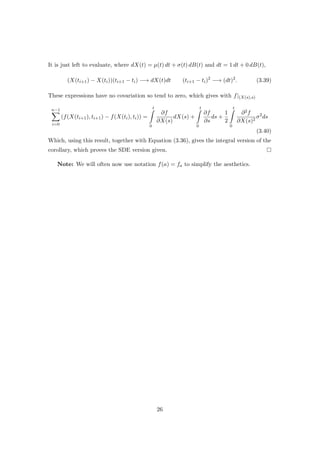
![4 Stochastic Differential Equations
A general SDE, as previously seen, only makes sense in the terms of It¯o integrals and
stochastic processes and is defined by:
Definition 4.0.1. For a stochastic process Y (t) with α(t) and γ(t) being Fti -measurable
with respect to Brownian motion B(t), a stochastic differential equation has the form
dY (t) = α(t, Y (t)) dt + γ(t, Y (t)) dB(t). (4.1)
There exists two types of solutions to SDE’s, know as ‘Strong’ and ‘Weak’ type.
4.1 Strong Solutions
Definition 4.1.1. As on [3, p. 137], A strong solution to an SDE is a stochastic
process Y (t) of the form
Y (t) = Y (0) +
t
0
α(u, Y (u)) du +
t
0
γ(u, Y (u)) dB(u), (4.2)
Subject to the following:
• Y is B(s) adapted, where s ≤ t.
• The integrals are well defined.
• Y is a function of B(t), α and γ.
Example 4.1. Geometric Brownian Motion
Similar to [7, Example 5.1.1], we take an SDE of the form
dXt = rXt dt + σXt dBt. (4.3)
This is motivated by looking at a typical model for rate of growth:
dXt
dt
= αtXt, X(0) = X0 (4.4)
But instead with a stochastic element Wt such that it has the properties of Wt = dBt
dt
(although we know Brownian Motion has no derivative, see 2.4.1) in a way which makes
αt = r + σWt. (4.5)
Now, using the It¯o formula for It¯o processes, Equation (3.28), on f(Xt) = ln(Xt).
27](https://image.slidesharecdn.com/3296b155-6d57-4931-bbc4-d7bce87ac5d8-150616142723-lva1-app6891/85/Stephens-L-28-320.jpg)
![Figure 7: Five realizations of Geometric Brownian Motion as compared to the grey
dashed curve being the standard growth model expectation.
Definition 4.1.2. As on [1, p. 129], for X(t) with SDE as in (4.1), the Stochastic
Exponential is known as U(t) = e(X), satisfying
U(t) = 1 +
t
0
U(s)dX(s). (4.10)
Definition 4.1.3. As on [1, p. 130], for U(t) with SDE as in (4.1), the Stochastic
Logarithm is known as X(t) = l(U), satisfying
X(t) = ln
U(t)
U(0)
+
1
2
t
0
d[U, U](S)
U2S
. (4.11)
Example 4.2. General Linear SDE’s:
To help us solve linear SDE’s of the form
dX(t) = (λt + µtXt) dt + (ϕt + ωtXt) dBt, (4.12)
we look at [1, p.132] and define X(t) as a function of two new parameters
Xt = UtVt U0 = 1, V0 = X(0), (4.13)
29](https://image.slidesharecdn.com/3296b155-6d57-4931-bbc4-d7bce87ac5d8-150616142723-lva1-app6891/85/Stephens-L-30-320.jpg)
![with
dUt = µtUt dt + ωtUt dBt (4.14)
and
dVt = at dt + bt dBt. (4.15)
Implementing the stochastic product rule, (Example (3.25))
dXt = UtdVt + VtdUt + d [U, V ]t = Ut(at dt + bt dBt) + VtUt(µt dt + ωt dBt) + Utωtbt dt
(4.16)
So, as UtVt = Xt
dXt = (Utat + Utωtbt + µtXt) dt + (Utbt + ωtXt) dBt, (4.17)
means that
Utat + Utωtbt = λt & Utbt = ϕt. (4.18)
Resulting in
at =
λt − ϕtωt
Ut
& bt =
ϕt
Ut
, (4.19)
hence making the solution to the SDE, as in [1, p.132 (5.31)]
Xt = Ut
X(0) +
t
0
λs − ϕsωs
Us
ds +
t
0
ϕs
Us
dBs
(4.20)
Example 4.3. Brownian Bridge
As in [1, (5.34) p.133] a “Brownian Bridge” is defined by the following SDE:
dXt =
b − Xt
T − t
dt + dBt, X(0) = a & X(T) = b for 0 ≤ t < T. (4.21)
First identifying the functions in terms of (4.12),
λt =
b
T − t
, µt = −
1
T − t
, ϕt = 1, ωt = 0.
Inputting them into our solution (4.20)
Xt = Ut
a +
t
0
b
Us(T − s)
ds +
t
0
1
Us
dBs
. (4.22)
So in finding Ut we can solve our equation
dUt = −
Ut
T − t
dt ⇒
1
Ut
dUt = −
1
T − t
dt ⇒ ln(Ut) = ln(AT − t)
30](https://image.slidesharecdn.com/3296b155-6d57-4931-bbc4-d7bce87ac5d8-150616142723-lva1-app6891/85/Stephens-L-31-320.jpg)
![implies
Ut = A(T − t), U0 = 1 ⇒ 1 = A · T ⇒ Ut =
(T − t)
T
.
Which makes (4.22)
Xt = (1 −
t
T
)a +
t
T
b + (T − t)
t
0
1
(T − s)
dBs for 0 ≤ t < T (4.23)
Evaluating the integral for the standard partition of {tn
i } in the interval [0, t], using the
definition of an Ito integral, our Brownian Bridge solution is
Xt = (1 −
t
T
)a +
t
T
b + (T − t)
n−1
i=0
1
(T − ti)
(Bti+1 − Bti ). (4.24)
Which the following graph is a realization of:
Figure 8: A realisation of a Brownian Bridge, pinned at (X, t) = (−1, 0) & (1, 1).
4.2 Weak Solutions
As in [1, Section 5.6] Weak solutions are solutions to an SDE in distribution, but on
another probability space
31](https://image.slidesharecdn.com/3296b155-6d57-4931-bbc4-d7bce87ac5d8-150616142723-lva1-app6891/85/Stephens-L-32-320.jpg)
![Definition 4.2.1. For a different filtration, ˜Y (t) and ˜B(t) if for all t our integrals are
defined and ˜Y (t) satisfies
˜Y (t) = ˜Y (0) +
t
0
µ(s, ˜Y (s)) ds +
t
0
σ(s, ˜Y (s)) d ˜B(s). (4.25)
Then ˜Y (t) is a solution of the SDE in the form denoted by 4.1.
Example 4.4. Tanaka’s Stochastic Differential Equation [1, Example 5.15]
dYt =
dBt Yt ≥ 0
−dBt Yt < 0.
(4.26)
Also known by introducing the function sign(x) to make the SDE:
dYt = sign(Yt)dBt (4.27)
Since, in our traditional SDE of the form in 4.1, γ = sign(Yt) is discontinous, we look for
weak solutions, because, as described in the existence of strong solutions in [1, Section
5.4], this discontinuity does not satisfy the conditions. Instead we take a t such that:
˜Yt =
t
0
dYt
sign(Yt)
, (4.28)
and see that ˜Yt is a Brownian motion in itself.
32](https://image.slidesharecdn.com/3296b155-6d57-4931-bbc4-d7bce87ac5d8-150616142723-lva1-app6891/85/Stephens-L-33-320.jpg)
![Figure 9: A realization of a solution to the Tanaka differential equation.
Forward equation
For general weak solutions of the differential equation of the form 3.33:
dX(t) = µ(X(t), t) dt + σ(X(t), t) dB(t)
With the use of [10, Pp.4] & [11, S.7] we firstly define L, such that
Lu(Xt) = lim
δt−→0
1
δt
(E [u(Xt+δt|Xt = x)] − u(x)) . (4.29)
Subsequently, if we introduce a ‘Transition Probability’ function P(x, t|x , t ) meaning
the probability the function goes from Xt = x to Xt = x
E [u(Xt+δt|Xt = x)] = u(y)P(y, t + δt|x, t) dy.
Manipulating the following part of Equation (4.29):
E [u(Xt+δt|Xt = x)] − u(x) = u(y)P(y, t + δt|x, t) dy − u(x),
by multiplying by P(x, t|x , t ) and integrating over x,
u(y) P(y, t + δt|x, t)P(x, t|x , t ) dx dy − P(x, t|x , t )u(x) dx. (4.30)
33](https://image.slidesharecdn.com/3296b155-6d57-4931-bbc4-d7bce87ac5d8-150616142723-lva1-app6891/85/Stephens-L-34-320.jpg)
![But, due to the memoryless (Markov) property of our stochastic process in question,
the probability of going from Xt = x to Xt = x and the probability of going from
Xt = x to Xt+δt = y over all x is the same as the probability of going from Xt = x to
Xt+δt = y (Chapman-Kolmogorov Theorem). Written formally as
P(y, t + δt|x, t)P(x, t|x , t ) dx = P(y, t + δt|x , t ).
So, we have, inputting this result in Equation (4.30) and re-entering that into Equation
(4.29) and changing the dummy variable y to x.
[Lu(x)] P(x, t|x , t ) dx = u(x) lim
δt−→0
1
δt
P(x, t + δt|x , t ) − P(x, t|x , t ) dx.
Evaluating the limit as a derivative
[Lu(x)] P(x, t|x , t ) dx = u(x)
∂P(x, t|x , t )
∂t
dx = u(x) L∗
P(x, t|x , t ) dx.
So equating inside the integral
∂
∂t
P(x, t|x , t ) = L∗
P(x, t|x , t ) (4.31)
As a result from Definition 3.4.1,for It¯o processes for a function u(Xt),
u(Xt+δt) = u(Xt) +
t+δt
t
du
dX
dX(s) +
1
2
t+δt
t
d2u
dX2
σ2
ds, (4.32)
where
t+δt
t
du
dX
dX(s) =
t+δt
t
du
dX
µ ds +
t+δt
t
du
dX
σ dB(s).
Then take the expectation of both sides of Equation (4.32)
E [u(Xt)] − u(X0) = E
t+δt
t
µ
du
dX
+
σ2
2
d2u
dX2
ds
+ E
t+δt
t
σ
du
dX
dB(s)
.
we know that
Eσ
du
dXs
dB(s) −→ 0
so
E [u(Xt+δt)| Xt = x] − u(Xt) = E
t+δt
t
µ
d
dX
+
σ2
2
d2
dX2
u(Xs) ds
.
Lu(Xt) = E µ
d
dX
+
σ2
2
d2
dX2
u(Xt) . (4.33)
34](https://image.slidesharecdn.com/3296b155-6d57-4931-bbc4-d7bce87ac5d8-150616142723-lva1-app6891/85/Stephens-L-35-320.jpg)
![Using a result from [11, S.7] which involves using integration by parts, if we have our L
in this form, then
L∗
· = −
d(µ·)
dX
+
1
2
d2(σ2·)
dX2
.
So, using this with Equation (4.31) and setting the notation P(x, t|x , t ) = p(x, t), we
obtain
The Fokker-Planck Equation
∂p
∂t
= −
∂(µp)
∂y
+
1
2
∂2(σ2p)
∂y2
(4.34)
For a stochastic process with no drift, we get the typical solution to the diffusion equa-
tion, given the initial condition is a delta function on x is, as in [11, S.7]:
p(x, t) =
1
√
2πt
e
−
x2
2t (4.35)
These solutions are known as ‘forward equations’ as they take an initial condition and
go in positive time increments. It is also possible, using ‘backward equations’ to attempt
to calculate initial states given a final state.
35](https://image.slidesharecdn.com/3296b155-6d57-4931-bbc4-d7bce87ac5d8-150616142723-lva1-app6891/85/Stephens-L-36-320.jpg)
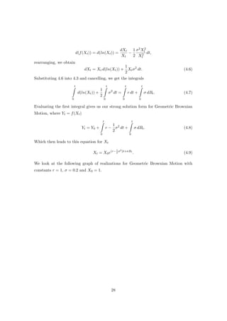
![5 Financial Applications
Modelling real world scenarios using elements of randomness is a technique used in
many fields. This project will focus on it’s financial applications, mainly the Nobel
Prize winning Black-Scholes model for pricing stock options, how it is derived and used.
5.1 Background
5.1.1 Stock Prices
Firstly, as in [1, p.291] there is a fundamental concept of ‘no arbitrage’ in asset pricing,
in which it is assumed that there are no opportunities in the market to make a risk-less
profit. With this concept in mind, if we imagine that, buying a stock S, which has no
randomness (volatility) returns the same amount as money placed in the bank, earning
the risk free rate of interest. With many complicated variables continually effecting stock
prices, one method to model them is to treat them as a stochastic process, namely, Ge-
ometric Brownian Motion (4.3). With the concept of the no arbitrage principle causing
a percentage ’drift’ component r for the equation
dSt = rSt dt. (5.1)
Also we incorporate a random element to the stock price by estimating the change in
daily returns on a stock to be of normal distribution, motivated by the following analysis:
Figure 10: The daily percentage returns on the Apple stock.
36](https://image.slidesharecdn.com/3296b155-6d57-4931-bbc4-d7bce87ac5d8-150616142723-lva1-app6891/85/Stephens-L-37-320.jpg)
![Using the method of testing for normality as described in [11, S.6] the table created
is used to see whether the gathered data is close enough to a standard normal to be
reasonably approximated as such. Where the largest absolute difference of our data
function away from the standard normal, as described in the source using the generally
accepted confidence interval, is
D1000 = 0.02665 < D1000,0.05 = 0.043007. (5.2)
We see the distribution adequately fits that of a standard normal with standard deviation
∼ 1.333%. So, dependant on it’s percentage volatility σ, including the drift as previously
described we generate an SDE for S in the form (4.3)
dSt = rSt dt + σSt dBt (5.3)
Which is the typical SDE for modelling stock prices in general. We will from now on,
for simplicity, assume r and σ to be constant unless otherwise stated. We have already
solved this equation in Example (4.1) and it results in a process of the form
St = S0e(r−1
2
σ2)t+σBt
. (5.4)
5.1.2 Options
Firstly, we will briefly look at what a stock option is, to understand how we can model
it’s price. There are two main types of ‘European vanilla’ stock options, namely a ‘call’
(and a ‘put’). They are contracts for the right, but not the obligation, to buy (or sell)
a stock S, for a ‘strike’ price E ‘exercised’ at a time T. You can have a ‘long’ or a
‘short’ position in these contracts, being the holder and the writer respectively. The
final ‘value’ at maturity is known as the pay-off and is dependant on the market value
of the stock at that time and whether you are in a long or short position, the pay-off
diagrams are as such:
38](https://image.slidesharecdn.com/3296b155-6d57-4931-bbc4-d7bce87ac5d8-150616142723-lva1-app6891/85/Stephens-L-39-320.jpg)
![Figure 12: The pay-off diagrams for a vanilla call and put at time T with strike E.
5.2 Black-Scholes
The option contract itself has a value throughout its lifetime, dependant on the likelihood
of the final pay-off, given the current stock price and time, which can be denoted as
V (S, t). Calculating V (S, t) needs to take into account many factors and one way to
model this was developed, as in [11, S.2] by “Fischer Black” and “Myron Scholes” in a
1973 paper, later expanded on by “Robert C. Merton” to a degree in which the work
done by all three granted a Nobel Prize in economics and is referred to today as the
“Black-Scholes option pricing model” which we will explore.
The equation used is derived, as in [8, Section 6], starting with a certain portfolio Π of
one long option of value V (S, t) as described and the purchase of delta (∆) of the stock
S (will mostly be fractional, something not usually to be possible, but it is assumed)
denoted by
Π = V − ∆S. (5.5)
39](https://image.slidesharecdn.com/3296b155-6d57-4931-bbc4-d7bce87ac5d8-150616142723-lva1-app6891/85/Stephens-L-40-320.jpg)
![Black-Scholes Equation Solution
Taking the general derivation for the Black-Scholes option pricing formula from [8, Sec-
tion 8.2], we make the following substitutions into the Black-Scholes Equation (5.12)
V = e−r(t−t)
U ⇒
∂U
∂t
+
1
2
σ2
S2 ∂2U
∂S2
+ rS
∂U
∂S
= 0
τ = T − t ⇒
∂U
∂τ
=
1
2
σ2
S2 ∂2U
∂S2
+ rS
∂U
∂S
ξ = log(S) ⇒
∂U
∂τ
=
1
2
σ2 ∂2U
∂ξ2
+ (r −
1
2
σ2
)
∂U
∂ξ
x = ξ + (r −
1
2
σ2
)τ & U = W(x, τ) ⇒
∂W
∂τ
=
1
2
σ2 ∂2W
∂x2
So we are looking to satisfy
∂W
∂τ
=
1
2
σ2 ∂2W
∂x2
. (5.13)
Observing the following function
W(x, τ) = F(τ)I(x, τ), (5.14)
where
F(τ) =
1
σ
√
2πτ
, I(x, τ) =
∞
−∞
e−
(x −x)2
2σ2τ Payoff(ex
)dx . (5.15)
We know by partial differentiation on Equation (5.14) with respect to τ
∂W
∂τ
=
∂F
∂τ
I + F
∂I
∂τ
. (5.16)
With the individual derivatives evaluated
∂F
∂τ
= −
1
2τ
F,
∂I
∂τ
=
∞
−∞
(x − x)2
2σ2τ2
e−
(x −x)2
2σ2τ Payoff(ex
)dx . (5.17)
Substituting (5.17) into (5.16)
∂W
∂τ
= −
1
2τ
FI + F
∞
−∞
(x − x)2
2σ2τ2
e−
(x −x)2
2σ2τ Payoff(ex
)dx .
Rearranging, results in
∂W
∂τ
=
1
2
σ2
F
∞
−∞
(x − x)2
σ4τ2
−
1
σ2τ
e−
(x −x)2
2σ2τ Payoff(ex
)dx
. (5.18)
41](https://image.slidesharecdn.com/3296b155-6d57-4931-bbc4-d7bce87ac5d8-150616142723-lva1-app6891/85/Stephens-L-42-320.jpg)
![We now look at 1
2σ2 multiplied by the second partial derivative of (5.14) with respect
to x
1
2
σ2 ∂2W
∂x2
=
1
2
σ2
F
∂2I
∂x2
. (5.19)
Evaluating the derivative
∂2I
∂x2
=
∞
−∞
(x − x)2
σ4τ2
−
1
σ2τ
e−
(x −x)2
2σ2τ Payoff(ex
)dx . (5.20)
Substituting (5.20) into (5.19)
1
2
σ2 ∂2W
∂x2
=
1
2
σ2
F
∞
−∞
(x − x)2
σ4τ2
−
1
σ2τ
e−
(x −x)2
2σ2τ Payoff(ex
)dx
. (5.21)
We notice that
∂W
∂τ
=
1
2
σ2 ∂2W
∂x2
.
So W(x, τ) satisfies the original equation. We look whether boundary conditions are
satisfied, namely
V (S, T) = Payoff(S) ⇒ W(x, 0) = Payoff(ex
).
But as W(x, τ) has a specially engineered Dirac delta function δ(x −x) = e
−
(x −x)2
2σ2τ
σ
√
2πτ
(See
[8, Equation 8.3]) which has the property
lim
τ−→0
W(x, τ) = lim
τ−→0
∞
−∞
δ(x − x)Payoff(ex
)dx = Payoff(ex
).
Satisfying the final conditions. See that substituting back in the variables redefined at
the beginning of the derivation, gives rise to the solution for a generic pay-off function
P(S), as in [8, p.176]
V (S, t) =
e−r(T−t)
σ 2π(T − t)
∞
0
e
−
log(S/S ) + (r − 1
2σ2(T − t))
2
2σ(T − t) P(S )
dS
S
. (5.22)
Black-Scholes Analysis
With the pay-off’s given in figure 12 We can write the more well known and concise
form for the Black-Scholes model for the value of a call as seen in [8, 8.2.1], by starting
with Equation 5.22, under the following conditions
For P(S) = max(S − E, 0), V (S, t) = C(S, t), ξ = log(S ), (5.23)
42](https://image.slidesharecdn.com/3296b155-6d57-4931-bbc4-d7bce87ac5d8-150616142723-lva1-app6891/85/Stephens-L-43-320.jpg)
![which means
C(S, t) =
e−r(T−t)
σ 2π(T − t)
∞
E
e
−
log(S) − ξ + (r − 1
2σ2(T − t))
2
2σ(T − t) (eξ
− E)dξ . (5.24)
After completing the square in one of the integrals, we arrive at
C(S, t) = SN(d1) + Ee−r(T−t)
N(d2), (5.25)
where
d1 =
ln(S/E) + (r + 1
2σ2)(T − t)
σ
√
T − t
, d2 =
ln(S/E) + (r − 1
2σ2)(T − t)
σ
√
T − t
,
with
N(x) =
1
√
2π
x
−∞
e−y2
2 dy.
We can test the real world reliability of this for our earlier AAPL stock, taking data
from [11, S.3, S.4], we can estimate the risk free interest rate r ≈ 0.11% and our stock
price volatility to be
Daily: Standard Deviation ≈ 1.33% ⇒ Variance ≈ 1.33%2
≈ 0.0178%,
Yearly: Variance ≈ 365 · 0.0178% ≈ 6.49% ⇒ Standard Deviation ≈
√
6.49% ≈ 25.5%.
Using the values of the Black-Scholes model with S = 124.95, r ≈ 0.11%, σ ≈ 25% &
T ≈ 0.58 of a year and option price data from [11, S.5] we see the comparison
Strike ($) 60 65 70 75 80 85 90 95 100
Market Data 68.2 66.32 53.55 49.4 44.3 38.4 35.3 30.5 26.75
B-S Model 64.99 59.99 55.00 50.02 45.07 40.18 35.39 30.76 26.35
Strike ($) 105 110 115 120 125 130 135 140 145
Market Data 22.45 18.82 15.4 12.5 10.1 7.92 6.2 4.75 3.6
B-S Model 22.25 18.49 15.13 12.19 9.67 7.57 5.84 4.44 3.34
Strike ($) 150 155 160 165 170 175 180 185 190
Market Data 2.7 1.95 1.47 1.11 0.8 0.65 0.46 0.39 0.31
B-S Model 2.48 1.82 1.33 0.95 0.68 0.48 0.34 0.24 0.16
This data represented diagrammatically looks like the following:
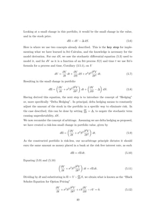
43](https://image.slidesharecdn.com/3296b155-6d57-4931-bbc4-d7bce87ac5d8-150616142723-lva1-app6891/85/Stephens-L-44-320.jpg)
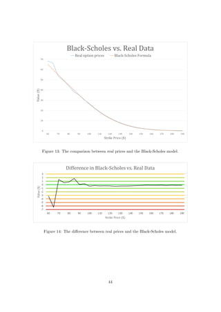
![[8, Section 8.9] using all the other values that we know in the Black-Scholes model and
equating it to the market value to reverse engineer the volatility measure, called “Implied
Volatility”. Using the ideas from the code on [8, p.192], we look at the volatility implied
by the market under the Black-Scholes model using the Newton Rahpson method, in
this case for when the B-S estimate is within $1 of the market value.
Figure 15: Graph showing the actual volatility which would achieve the market value
under the Black-Scholes model for varying strike prices.
This reinforces the idea that the selection of a constant volatility for all strike prices
in Black-Scholes estimates cannot be achieved. All other parameters have remained
constant here, with the only variable being the strike price, and volatility is not constant.
This could be grounds for interpreting some strike price dependency for the volatility
measure to account for the market behaviour. The reason our B-S estimate is somewhat
accurate however, is because there is not much variation in volatility so a constant
assumption does not fair too badly.
There is also no guarantee that a stock will act in a way it has done previously, we
can only make estimations on its future behaviour using past data.
Risk Free Rate
We have also assumed a constant risk free rate, which again is not necessarily true, but
is relatively fair for small time periods as there is not a huge amount of variation. We
look at data from [11, S.3] to see the change in r:
46](https://image.slidesharecdn.com/3296b155-6d57-4931-bbc4-d7bce87ac5d8-150616142723-lva1-app6891/85/Stephens-L-47-320.jpg)

![7 Summary & Extensions
To summarize, I believe the ideas as a result of stochastic calculus are a great tool in
helping understanding an modelling processes, especially that which would be allowed
to naturally occur without the awareness of its implementation. Stochastic calculus is
used in population modelling, which is not covered in this project but is an extension
of the ideas presented (See [9], or [10, Pp.2]).
But any widely renowned solution to a problem influenced by human behaviour
using uncertainty can be subsequently taken advantage of and exploited by making
the assumption that the human aspect of the system will now behave according the
“Solution”, as I believe what is happening to an extent in the Black-Scholes model.
In reference to the Black-Scholes model, it has more uses than just the equation
derived here, it is used for the pricing of many types of options different to our “Vanilla”
call. It is also used for the described “put”, also binary versions of the call and put,
options on stocks with dividend payments, and a variety of other “Exotic” options, many
of which can be seen and researched further in [8]. However, Black-Scholes is not the
exclusive idea for modelling stock prices, there are other ideas such as the idea of chaos
theory implementation, see [10, Pp.3].
There is also the concept of “The Stratonovich Integral” which instead takes the
midpoint of the interval like outlined and more in [3, Section 2.4], which is another way
of looking at stochastic calculus which can be explored.
The main things to note about It¯o calculus is where it differs from general concepts of
regular calculus we are familiar too. Like the definition of the integral (Eq.(3.10)) , the
product rule/integration by parts (Eq.(3.25)), the exponential and logarithm (Eq.(4.10)
& (4.11)) and the concept of strong (Eq.(4.2)) and weak (Eq.(4.25)) solutions.
48](https://image.slidesharecdn.com/3296b155-6d57-4931-bbc4-d7bce87ac5d8-150616142723-lva1-app6891/85/Stephens-L-49-320.jpg)
![References
[1] Klebaner, F. C. (2012) Introduction to Stochastic Calculus with Applications, 3rd
Edition, Imperial College Press.
[2] Rogers, LCG. & Williams D. (1987) Diffusions, Markov Processes, and Martingales,
Volume 2: It¯o Calculus, John Wiley & Sons.
[3] Mikosch, T. (1998) Elementary Stochastic Calculus, with Finance in View,
Advanced Series on Statistical Science & Applied Probability Volume 6, World
Scientific.
[4] Jones, P. W. & Smith, P. (2010) Stochastic Processes, An Introduction,
2nd Edition, CRC Press.
[5] Franchi, J. & Le Jan, Y. (2012) Hyperbolic Dynamics and Brownian Motion, An
Introduction,
1st Edition, Oxford University Press.
[6] Papoulis, A. (1984) Probability, Random Variables, and Stochastic Processes,
2nd Edition, McGraw-Hill International Editions.
[7] Øksendal, B. (2013) Stochastic Differential Equations, An Introduction with Appli-
cations,
6th Edition, Springer.
[8] Wilmott, P. (2007) Paul Wilmott Introduces Quantitative Finance,
2nd Edition, Wiley.
[9] Etheridge, A. (2012) Some Mathematical Models from Population Genetics,
Lecture notes in Mathematics, Springer-Verlag Berlin Heidelberg.
[10] Papers:
Pp.1 Dunbar, S. R.
Stochastic Processes and Advanced Mathematical Finance,
Quadratic Variation of the Wiener Process
University of Nebraska-Lincoln
http://www.math.unl.edu/~sdunbar1/MathematicalFinance/Lessons/
BrownianMotion/QuadraticVariation/quadraticvariation.pdf
49](https://image.slidesharecdn.com/3296b155-6d57-4931-bbc4-d7bce87ac5d8-150616142723-lva1-app6891/85/Stephens-L-50-320.jpg)
![Pp.2 Braumann, C. A.
Population Growth in Random Environments:
Which Stochastic Calculus?
Bulletin of the International Statistical Institute, LXII
http://dspace.uevora.pt/rdpc/bitstream/10174/1309/1/
Braumann-Proc%2056%20ISI-07.pdf
Pp.3 Abraham, A., Philip, N. S. & Saratchandran, P.
Modeling Chaotic Behavior of Stock Indices Using Intelligent Paradigms
Oklahoma State University, Cochin University of Science and Technology &
Nanyang Technological University http://arxiv.org/ftp/cs/papers/0405/
0405018.pdf
Pp.4 Lyons, S.
Introduction to Stochastic Differential Equations
http://homepages.inf.ed.ac.uk/s0978702/introsde.pdf
[11] Websites:
S.1 Wolfram: Normal Distribution,
http://mathworld.wolfram.com/NormalDistribution.html
S.2 Wikipedia: Black Scholes Model,
http://en.wikipedia.org/wiki/Black%E2%80%93Scholes_model
S.3 USA federal reserve annual risk free rate data,
http://www.federalreserve.gov/releases/h15/data.htm
S.4 Yahoo finance: Apple Inc. stock price history,
http://finance.yahoo.com/q/hp?s=AAPL+Historical+Prices
S.5 Yahoo finance: Apple Inc. option prices,
http://finance.yahoo.com/q/op?s=AAPL+Options
S.6 Kolmogorov-Smirnov-Test Detail,
http://www.real-statistics.com/tests-normality-and-symmetry/
statistical-tests-normality-symmetry/kolmogorov-smirnov-test/
S.7 Wikipedia: Fokker Planck Equation,
http://en.wikipedia.org/wiki/Fokker%E2%80%93Planck_equation
50](https://image.slidesharecdn.com/3296b155-6d57-4931-bbc4-d7bce87ac5d8-150616142723-lva1-app6891/85/Stephens-L-51-320.jpg)


The document provides an introduction to Itô calculus, which is a form of stochastic calculus used to model environments with unpredictability. It begins by establishing foundations in ordinary calculus, probability theory, and stochastic processes. This includes definitions of integrals, random variables, density/distribution functions, expectations, and Brownian motion. The document then covers the key concepts of Itô calculus, such as the Itô integral, Itô's formula, and Itô processes. It discusses how these allow modeling via stochastic differential equations. Finally, it explores applications of Itô calculus in financial modeling, particularly the Black-Scholes option pricing model.